Contents

% bpdq_demo_1d : Demo for BPDQ reconstruction in 1-d
%
% This demo first creates a random, sparse 1-d signal, creates a gaussian
% random sensing matrix, and computes the quantized measurements.
%
% Then the BPDQ algorithm is run to reconstruct the signal from the quantized
% measurements.
%
% For Comparison, BPDN (corresponding to p=2) is also run, then the results
% from both reconstruction programs are compared.
%
% Plots of relative errors ( ||x_n - x_(n-1)||/||x_n|| )
% as a function of iteration number are given to demonstrate empirical
% convergence of the douglas-rachford algorithm used to compute the
% BPDQ program.
%
% This demonstrates the method described in
% "Dequantizing Compressed Sensing : When Oversampling and Non-Gaussian
% Constraints Combine"
% by Laurent Jacques, David Hammond, M. Jalal Fadili
% ( submitted to IEEE Transactions on Signal Processing)
%
% This file is part of BPDQ Toolbox (Basis Pursuit DeQuantizer)
% Copyright (C) 2009, the BPDQ Team (see the file AUTHORS distributed with
% this library) (See the notice at the end of the file.)



% Note: With parameters as set in this demo, execution time was 18 seconds
% on 2.4 GHz Intel Core 2 Duo processor.

Experiment Setup and Demo Parameters :

Note: Quantization threshold alpha is computed depending on nbins and on the signal instance)

N=1024;
K=16;
M=K*25;
p=4;
nbins=10;

Parameters for controlling BPDQ algorithm.

The Douglas-Rachford algorithm parameters * dr_lambda must be between 0 and 2, dr_gamma must be positive. * dr_gamma and dr_lambda are described in Jacques et. al. section IV-A; dr_lambda corresponds to alpha_t in equation 10

Note : a priori these parameters could vary at each iteration, in this code they are kept constant.

dr_verbosity and fca_verbosity control output of information about speed of convergence at each iteration, set to 0 to supress output, to 1 to show output. See: bpdq_d_r_iter.m and bpdq_prox_f_comp_A.m for details.

Other options * dr_maxiter, dr_relerr_thresh, fca_maxiter, fca_relerr_thresh are defined in in control_params in bpdq_1d.m, see bpdq_1d.m for details.

bpdq_opts={'dr_gamma',.05,'dr_lambda',1.5,'dr_verbosity',0,'fca_verbosity',0};

Create signal and sensing matrix

fprintf('Generating signal of length N=%g and sparsity K=%g\n',N,K);
x=bpdq_generate_1d_signal(N,K);

fprintf('Generating sensing matrix for M=%g random measurements\n',M);
A=bpdq_generate_sensing_matrix(M,N);

Generating signal of length N=1024 and sparsity K=16
Generating sensing matrix for M=400 random measurements

Compute measurements and quantize

fprintf('Computing quantized measurements with %g quantization levels\n',nbins);
y=A*x;
alpha = 2.01*norm(y, Inf)/nbins;
yq = bpdq_quantize(y, alpha);

Computing quantized measurements with 10 quantization levels

Call BPDQ decoder

% Let's first compute apropriate epsilon (ref Jacques et. al section III-C)
epsilon=bpdq_err_p(p,alpha,M);
fprintf('Running BPDQ reconstruction with p=%g\n',p);
[x_bpdq,D_bpdq] = bpdq_1d(yq,A,epsilon,p,bpdq_opts{:});

Running BPDQ reconstruction with p=4

Compare to BPDN

epsilon2=bpdq_err_p(2,alpha,M);
fprintf('Running BPDN (p=2) reconstruction\n');
[x_bpdn,D_bpdn]  = bpdq_1d(yq,A,epsilon2,2,bpdq_opts{:});

Running BPDN (p=2) reconstruction

Examine results

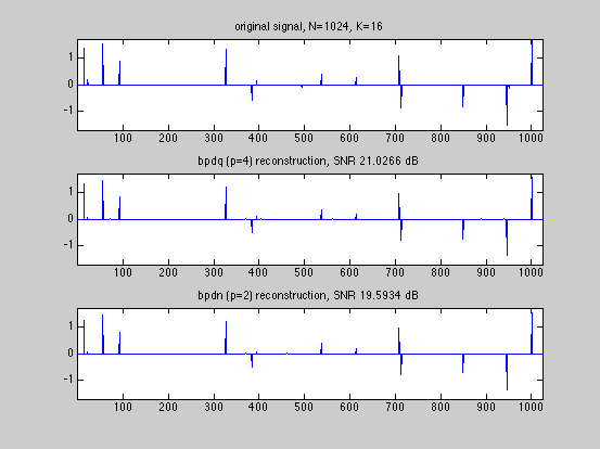
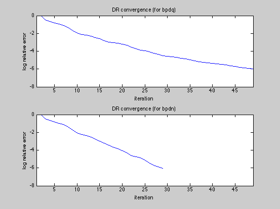
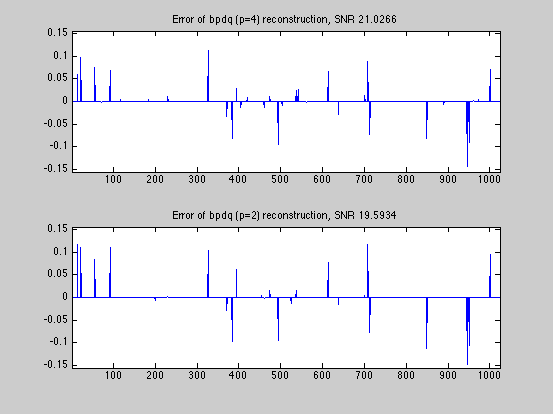
SNR_bpdq = bpdq_compute_snr(x,x_bpdq);
SNR_bpdn = bpdq_compute_snr(x,x_bpdn);

fprintf('Displaying results and convergence curves\n');
% plot results and convergence curves

dmax=1.05*max(abs([x(:);x_bpdq(:);x_bpdn(:)]));
fig1ylim=[-dmax,dmax];
fig1xlim=[1,numel(x)];
figure(1)
subplot(3,1,1);
tstr=sprintf('original signal, N=%g, K=%g',N,K);
plot(x);
xlim(fig1xlim);
ylim(fig1ylim);
title(tstr);

subplot(3,1,2);
tstr=sprintf('bpdq (p=%g) reconstruction, SNR %g dB',p,SNR_bpdq);
plot(x_bpdq);
xlim(fig1xlim);
ylim(fig1ylim);
title(tstr);

subplot(3,1,3);
tstr=sprintf('bpdn (p=2) reconstruction, SNR %g dB',SNR_bpdn);
plot(x_bpdn);
xlim(fig1xlim);
ylim(fig1ylim);
title(tstr);

figure(2)
subplot(2,1,1)
fig2xlim=[1,max(numel(D_bpdq.dr_relerr_save),...
          numel(D_bpdn.dr_relerr_save))];
plot(log10(D_bpdq.dr_relerr_save));
xlim(fig2xlim);
title('DR convergence (for bpdq)');
xlabel('iteration');
ylabel('log relative error');

subplot(2,1,2)
plot(log10(D_bpdn.dr_relerr_save));
xlim(fig2xlim);
title('DR convergence (for bpdn)');
xlabel('iteration')
ylabel('log relative error');

figure(3)
diff_bpdq=x-x_bpdq;
diff_bpdn=x-x_bpdn;
dmax=1.05*max([abs(diff_bpdq);abs(diff_bpdn)]);
fig3ylim=[-dmax,dmax];
fig3xlim=[1,numel(x)];
subplot(2,1,1);
tstr=sprintf('Error of bpdq (p=%g) reconstruction, SNR %g',p,SNR_bpdq);
plot(diff_bpdq);
xlim(fig3xlim);
ylim(fig3ylim);
title(tstr);

subplot(2,1,2);
tstr=sprintf('Error of bpdq (p=2) reconstruction, SNR %g',SNR_bpdn);
plot(diff_bpdn);
xlim(fig3xlim);
ylim(fig3ylim);
title(tstr);

% The BPDQ Toolbox is free software: you can redistribute it and/or modify
% it under the terms of the GNU General Public License as published by
% the Free Software Foundation, either version 3 of the License, or
% (at your option) any later version.
%
% The BPDQ Toolbox is distributed in the hope that it will be useful,
% but WITHOUT ANY WARRANTY; without even the implied warranty of
% MERCHANTABILITY or FITNESS FOR A PARTICULAR PURPOSE.  See the
% GNU General Public License for more details.
%
% You should have received a copy of the GNU General Public License
% along with The BPDQ Toolbox.  If not, see <http://www.gnu.org/licenses/>.

Displaying results and convergence curves

Published with MATLAB® 7.7