Machine Learning and Language Processing Algorithms

For being able to cleanly process data, we defined a common format to use that was already previously explained. In this section, we just describe briefly the structure of such a .json file for using purpose. Such a file for crosswords contains multiple entries with the following fields :

In this section, we describe the model that we used to represent the definitions we gather. The bag-of-word model is a model for which the text is divided in a set of words that it is composed of but it still keeps track of the multiplicity of each word in the text. More useful information can be found here.

 

Dictionary:

 

In this chapter, we analyze different machine learning algorithms and compare them with our adjacency matrix model presented in Chapter \ref{chapter:ml}. We compare Naive Bayes and Decision Tree classifiers based on different feature sets and dimensionality reduction and feature extraction techniques using Spark's machine learning library (MLlib) \cite{sparkmllib}. Our goal is to test how the proposed adjacency matrix model performs comparing to the available state-of-the-art machine learning algorithms to solve the crosswords.

 

 

 

In this section, we define how we model our problem as a classification problem. As shown in Section \ref{section:definition}, our data is composed of a set of lines, where each line contains a word that needs to be predicted by the crossword solver, and a set of words that are related to the to-be-predicted word, i.e., the definition words. We have defined the classification problem as setting the words to be predicted as class labels, and the definition words as features. We define two different feature sets over the definition words.

 

 

In this section, we explain the feature sets that we have used to train the machine learning algorithms, and present the results we get with different feature sets and classification algorithms. We have tried two different feature sets, (i) stemmed definition words and (ii) letter frequencies, and two different classifiers (i) Naive Bayes and (ii) Decision Tree. In the following sections, we explain the two features sets we used, and present the results for using these feature sets with different classifiers.

 

In the first feature set, we use the weights of the stemmed definition words directly from the adjacency matrix as a feature vector for each to-be-predicted word. That is, for each word, there is one sparse feature vector including the weights of the word's definition words. For example, assume that in our dataset we have "CAT" as a word and its definition includes ("ANIMAL","DOG","HATE"), then the word "CAT" will have unique integer id as its classification label, and its features will be the whole row of the word "CAT" including the non-zero weights for the words "ANIMAL","DOG" and "HATE", and everything else as zero. Hence, the total length of each feature vector is actually the total number of unique words in our dataset with a lot of zero elements, a few non-zero elements. We keep the adjacency matrix in a sparse matrix.

 

Once we simply tried to feed these features to the Naive Bayes and Decision Tree classifiers, as expected, we got out of memory errors since the total number of features are the number of unique words in the adjacency matrix, which is around $600K$. To solve the problem of the large number of features, we tried dimensionality reduction and feature extraction techniques, which we have explained in the following sections.

 

First, we tried principal component analysis (PCA) as the dimensionality reduction technique. Principal component analysis transforms the space of the data so that the first coordinate of the transformed space has the largest variance of the data, the second coordinate of the transformed space has the second largest variance of the data, and so on. The principal components are the coordinates of the rotated space. Thereby, principal component analysis aims to reduce the dimensionality of the data to a small number of dimensions that can cover most of the variance of the data. In the best case, most of the variance are covered by the first principal component and the variance decreases rapidly along the principal components \cite{pcawiki}. We use Sparks PCA methods \cite{pcaspark} whose code snippet is as following.

 

    val tempDataToReduce: RowMatrix = new RowMatrix(data)

    val pcs: Matrix = tempDataToReduce.computePrincipalComponents(1000)

    val reducedData: RowMatrix = tempDataToReduce.multiply(pcs)

 

Line 1 creates a RowMatrix from the data we have, Line 2 computes the top 1000 principal components of the data, and lastly Line 3 projects the data to the space spanned by the top 1000 principal components. Observe that, if the size of the data is $N \times M$, then the size of the reducedData is $N \times 1000$ as we reduced the dimensionality from $M$ to $1000$. Once we run this code snippet in the cluster, however, we got out-of-memory error at Line 1. The reason is, while we keep the data as a sparse matrix, Spark constructs a dense matrix once we create the RowMatrix tempDataToReduce from the sparse matrix data. This gives an out-of-memory error since the size of the dense matrix is $600K \times 600K$. 

 

Therefore, we searched for a PCA method that can operate on sparse/very large matrices and decided to try the probabilistic principal component analysis (PPCA) proposed by \cite{pcaPaper, pcaCode}.  PPCA is designed for very large matrices such as gene expression datasets where the number of variables are in the orders of $10K$'s. PPCA uses Expectation Maximization (EM) to find the principal components. Our plan was 

 

 

1 Save the data into a text file within Spark

2 Read the data with MATLAB

3 Process the data with MATLAB and reduce the dimensionality

4 Read the data with Spark, and use the reduced data to train the classifiers

 

Hence, we saved the data as a text file in Spark, and parsed it with MATLAB, and run PPCA over the parsed data file. 

 

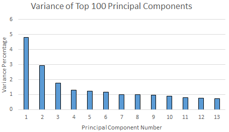
When we run PPCA on our dataset for the top 2 principal components, we get the results in less than 1 minute. However, the total variance of the first two principal components covers only $4.8245 + 2.9421 = 7.77 \%$ of the total variance of the data. Next, we increased the number of principal components to 20, which is finished in about 10 minutes. Figure \ref{fig:pcavar} shows the variance of the top 20 principal components. This time, the total variance of the top 20 principal components increases to only $24.16 \%$, and the variance covered by a principal component is quickly decreasing to less than $0.8 \%$. This means even if we get top 100 principal components, we may end up covering only $50 \%$ of the variance. Moreover, when we try to increase the number of principal components to $100$, we waited around $1$ hour and the PPCA algorithm was still not finished. Therefore, we decided to try another dimensionality reduction technique.

 

 

Since, the PPCA methodology did not satisfy our requirements, we decided to use the tf-idf feature extraction method. Given a corpus composed of a set of documents, tf-idf measurement of a word presents how much each word is important for each document. It is simply the multiplication of term frequency (tf) and inversed document frequency (idf) of each word. Tf measures how many times a word has appeared in its document, and idf measures in the inverse of how many documents, this word has appeared. Tf value alone can be misleading. Because words like "the", "or", "and" can appear a lot of time within a document, but does not carry a lot of information about the characteristics of the document. Idf metric balances the tf metric, since it divides the tf by the number of documents that the word has appeared showing that how much each important particularly for each document \cite{tfidfwiki}.

 

Although it is commonly used for document classification, we adapted tf-idf for our "word" classification problem. The classification problem translates into our case such that the document classes are the to-be-predicted crossword words, and the words of that document is the definition words of our dataset. We use Spark's available tf-idf measurement methodologies \cite{tfidfspark}. It simply takes the RDD of Seq(String)'s composed of the definition words, and returns the tf-idf value for each definition word. Once we get all the tf-idf values in the complete dataset, we had two options to reduce the dimensionality. The first one is to the select the top $N$ words with highest tf-idf values for each definition separately. That is, if a definition has $10$ words, we reduce the words in this definition to the set of words having top $5$ tf-idf values. Thereby, we reduce the number of words at each definition to at most $N$, i.e., to $5$ for the given example. The important point here is the fact that, even though we reduce the total number of features for each word to $5$, the total number of features across the whole dataset is still large. Once we apply this feature extraction, the total number of features reduced to $20K$, which was still large enough to create an out-of-memory error.

 

Hence, we decided to reduce the total number of features with a hard limit. That is, we collect all of the tf-idfs of the definition words, and take only the top $N$ of the complete set of words, and ignore any word in the dataset whose tf-idf value is less than the top $N$ tf-idf values. When, we apply this method with $N=10K$, we again got out-of-memory error after $3$ hours of running. Then, we reduce our dataset to its $1 \%$ which is $50K$ word-definition lines with $N=10K$. We again got out-of-memory error. Next, we reduced our dataset to its $0.1 \%$ which is $5K$ word-definition lines with $N=1K$. However, we again got out-of-memory error. Since, despite the fact that we reduced our dataset to as small as its $0.1 \%$ with only top $N=1K$ features (out of $600K$ ones), we got out-of-memory error, we decided to leave using the word-based feature approach where we used directly the weights from the adjacency matrix. We decided to find another way of defining the features over the definition words, which explain in the following section.

 

Note that for out-of-memory errors, we typically increased the amount of memory of executors to $70GB$ while the cluster is empty (during the nights), which did not help to mitigate the out-of-memory error. And this is valid for all of the out-of-memory errors we refer throughout the report.

 

Since we suffered a lot from large number of features based on word-based features, we decided to change our feature definitions. This time, we decided to count the number of frequencies of letter in the word definitions as features. That is, each to-be-predicted words from the crosswords are still the classes, however, we define the feature vector for each to-be-predicted word as the frequency of each letter in its definition. For the same example of the word "CAT" whose definition is ("ANIMAL","DOG","HATE"), we extract the feature as (3,0,0,1,1,0,1,1,1,0,0,1,1,1,1,0,0,0,0,1,0,0,0,0,0,0) whose length is $26$ as the size of the English alphabet, and each feature includes the number of times each letter appeared in the definition in the order of the English alphabet, 'A', 'B', 'C', ..., 'Z'.

 

Since, this time the number of features is only $26$, we did not need to use dimensionality reduction or feature extraction techniques to reduce the number of features. We tried these letter frequency features with Naive Bayes and Decision Tree classifiers, which we have explained in the following sections. 

 

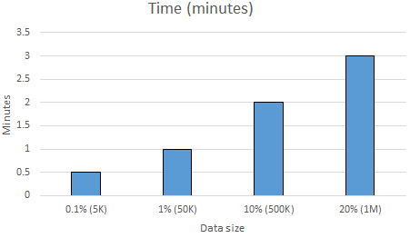
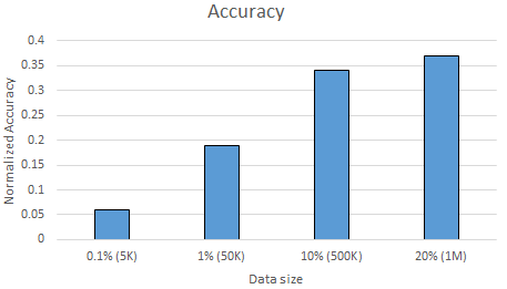
Although our data was reduced greatly thanks to our new features, we still got out-of-memory errors with Naive Bayes classifiers with the complete dataset. Hence, this time we gradually increased the size of our data until we got out-of-memory error, and measure the accuracy of Naive Bayes classifier with the letter frequency features as well as the time it requires to train and test the classifier. Figure \ref{fig:nbtime} and \ref{fig:nbacc} show the normalized accuracy and the amount of time it takes to train and test the Naive Bayes classifier as the amount data increases. Note that, we use $80\%$ of the data as training and $20\%$ of the data test data in all of our experiments. 

 

As shown by the x-axis of Figure \ref{fig:nbtime} and \ref{fig:nbacc}, we do not have any results after $20\%$ of the data, which is around $1M$ word-definition lines, as we got out-of-memory error. Figure \ref{fig:nbtime} shows that the time it requires to train and test the classifier increases as the data size increases. Moreover, training and testing $20\%$ of the complete data takes only $3.5$ minutes. This is very promising since with the previous feature set that we explain in Section \ref{sect:featureset1}, it was taking at least $1$ hour to only finish the feature extraction phase, or to get the out-of-memory error during the learning phase. Having only $3.5$ minutes provided us a lot more opportunities analyze the classifier.

 

As Figure \ref{fig:nbacc} shows, as we increase the data size, the accuracy increases as well. The accuracy gets to $0.37$ (over $1.0$) with $20\%$, $1M$ lines of word-definition. Although $0.37$ of accuracy is not very promising, it shows that Naive Bayes classifier is encouraging for solving the crosswords. Moreover, the accuracy increases as the data size increases is encouraging as well since it shows, in case of having more than only $20\%$ of the data set, we might actually get better accuracy. 

 

 

 

 

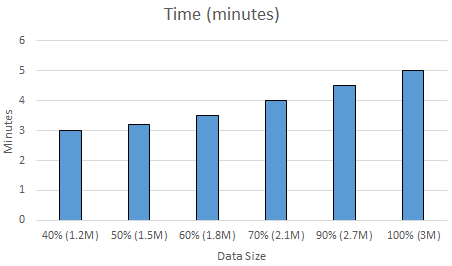
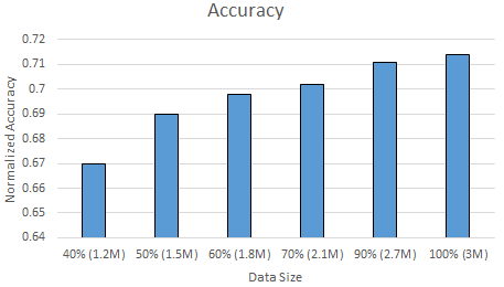
Using Only Crosswords: Therefore, next, we analyzed our dataset a bit in more detail. This time we reduced our dataset not randomly, but removing everything but the crosswords. As shown in Section \ref{section:definition}, our data includes word-definition lines from real crosswords as well ass from the Wiktionary dataset, where a definition of a word can be an example/synonym/etc.. of the word from the Wiktionary. Since our ultimate goal is to solve crosswords, we decided to exclude all the Wiktionary data, and use only the crossword dataset to train and test our Naive Bayes classifier with letter frequencies features. Thereby, we reduce the total data size to $50\%$. Next, again, we gradually increased the data size from $40\%$ to $100\%$ of all the crosswords, and measured the accuracy and time it takes to train and test the classifier. Figure \ref{fig:nbtimecw} and \ref{fig:nbacccw} shows the normalized accuracy and the amount of time it takes to train and test the Naive Bayes classifier as the amount data increases by using only the crossword data. Note that, we again use $80\%$ of the data as training and $20\%$ of the data test data in all of our experiments.

 

This time, unlike the case when we use the complete dataset including the Wiktionary data, we managed to train and test the Naive Bayes classifier without using by using the $100\%$ of the crossword dataset without getting an out-of-memory error. This is interesting. Because, when we use the complete dataset, more than $1M$ lines of word-definitions caused an out-of-memory error. However, when we use only the crossword data, we managed to use $3M$ lines of word-definitions, which is the complete crossword dataset we have. We think that the reason for that is the coherency of the dataset we use. When we mix the crosswords and Wiktionary datasets, the classifier gets needed to train itself for much more different cases as the crosswords and Wiktionary data actually represents different semantics. When we reduce the dataset only to the crossword data, the classifier is able to capture the semantics of the data by using less concise data which requires less amount of memory.

 

Figure \ref{fig:nbtimecw} shows that the amount of time it requires to train and test the classifier increases as the data size increases. Moreover, it is only $5$ minutes to train the complete $3M$ lines of crossword dataset, which is quite fast similar to the results shown in Figure \ref{fig:nbtime}. 

 

When we look at the accuracy results of the Naive Bayes classifier with only crosswords dataset shown by Figure \ref{fig:nbacccw}, we observe that the accuracy increases the data size increases from $1.2M$ to $3M$. Moreover, its $0.67$ for $40\%$ of the complete crossword dataset and increases to $0.71$ when we use the complete crossword dataset. This is a very promising result. By counting the letter frequencies in each definition, and using only the crossword dataset, we are able to achieve $71\%$ accuracy within only $5$ minutes of building the dataset, extracting the features, training and testing the classifier. The accuracy was only $37\%$ when we mix the crosswords and Wiktionary dataset (as shown in Figure \ref{fig:nbacc}), which was almost the half of the accuracy that we got by using only the crossword data. Therefore, we conclude that Naive Bayes classifier works well for solving the crosswords as it provide fast solutions with high accuracies if we use only the crosswords to train and test the dataset. Moreover, though increasing the training dataset is typically a good thing, we get $2x$ better accuracy when we use only the crossword dataset to train and test the Naive Bayes classifier.

 

 

 

To be able to explore if we can do better than $71\%$ accuracy with another classification algorithm, we also tried to use Decision Tree classifier with the letter frequency features. Since we got $2x$ better accuracy when we exclude the Wiktionary data and use only the crossword data with Naive Bayes classifier, we used only crossword data with Decision Tree as well. Although we were able to use Niave Bayes classifier with the complete crosswords data without getting an out-of-memory error, we did get out-of-memory error with Decision Tree classifier when we use the complete crossword dataset. Therefore, we gradually increased data size by also playing with several tuning parameters of the Decision Tree until we got an out-of-memory error.

 

Decision Tree has two main tuning parameters, maximum number of level that the tree will grow, i.e., maxDepth, and maximum number of bins that affect the maximum number of splits during the growth of the Decision Tree, i.e., maxBins. As we gradually increased the data size, we also played with these parameters to explore their affect on the classification and the accuracy. Table \ref{table:dt} shows the results. It has five columns where the first three columns presents the configuration of the test case, i.e., the data size, the maxDepth and maxBins, and the last two columns show the accuracy we get from the Decision Tree and the amount of time it requires to train and test the Decision Tree for the given configurations. The accuracy of the configurations that we got out-of-memory error has not been specified, i.e., '- symbol is placed in the field of accuracy. Note that, we again use $80\%$ of the data as training and $20\%$ of the data test data in all of our experiments.

 

The first thing to notice in Table \ref{table:dt} is the amount of time it requires to train and test the Decision Tree. It requires more than 4 hours to train the Decision Tree with $70\%$ of the data when we set $maxDepth = 20$, and $maxBins = 16$ (Line 4), and with a resulting accuracy of only $16\%$. If we decrease the $maxDepth$ to 5 and increase the $maxBins$ to 32 with $50\%$ of the data (Line 1), though it finishes in $7$ minutes, its accuracy reduces to only $3\%$, which is too low. When we increase the $maxDepth$ to 10 and decrease the $maxBins$ to 16 with again $50\%$ of the data (Line 2), we can only increase the accuracy to $7\%$ in $23$ minutes, which is not very fast. When we tried to increase the data size to $80\%$ with $maxDepth$ as 5 and $maxBins$ as 32 (Line 6), we again get only $3\%$ accuracy. Lastly, when we try to increase when we increase the maximum depth of the tree to more than 20 and increase the maximum number of bins to more than 16, we get out-of-memory error after waiting almost $7$ hours (Line 5). As we have shown in Section \ref{sect:nblc}, we were able to get $71\%$ accuracy in only $5$ minutes by using the $100\%$ of the crossword dataset with Naive Bayes classifier. Therefore, we conclude that, for our task Decision Tree is not an appropriate classifier since it requires a lot of time to train the classifier with a very low accuracy results.

 

Please see the LetterFeaturesDecisionTree.scala file under crosswords/app/src/main/scala/crosswords/spark/ for the implementation of this feature set technique with Decision Tree classifier.

 

\begin{table}

    \centering

  \begin{tabular}{| c | c | c | c | c | }

    \hline

    Data Size & maxDepth & maxBins & Accuracy & Time \\ \hline

    $50\% (1.5M)$ & 5 & 32 & 0.03 & $7min$ \\ \hline

    $50\% (1.5M)$ & 10 & 16 & 0.07 & $23min$ \\ \hline

    $50\% (1.5M)$ & 20 & 32 & - & $>1h$ \\ \hline

    $70\% (2.1M)$ & 20 & 16 & 0.16 & $4h17min$ \\ \hline

    $70\% (2.1M)$ & 30 & 32 & - & $>7h$ \\ \hline

    $80\% (2.4M)$ & 5 & 32 & 0.03 & $12min$ \\ \hline

  \end{tabular}

   \caption{The accuracy results and the time it requires to train and test the Decision Tree with letter frequencies using only the crossword data.}

  \label{table:dt}

\end{table}

 

 

 

Next, we wanted to explore if we can improve our Naive Bayes classifier further with a different set of features. This time instead of taking frequency of each letter in the definition of the words as feature vectors, we take the tf-idf values of each letter in the definition of the words. That is, if the word is "CAT" and its definition is ("ANIMAL","DOG","HATE"), we convert its definition into a string array where each string is one single letter, i.e., ("A", "N", "I", "M", "A", "L", "D", "O", "G", "H", "A", "T", "E"). We do this for the complete dataset. Then, we calculate the tf-idf value for each letter in the definitions and use directly them as features to feed into the Naive Bayes classifier. 

 

Since we already know that we can use the complete crossword data without getting an out-of-memory error, we directly used the $100\%$ of the crosswords. We again use $80\%$ of the data as training and $20\%$ of the data test data in all of our experiments. When we feed the tf-idf features of the letters to the Naive Bayes classifier, we got $55\%$ accuracy in 5 minutes. This is a lower accuracy value than the one that we used letter frequencies with the Naive Bayes classifier shown in Section \ref{sect:nbcl}, which was $71\%$. The reason for having lower accuracy with tf-idf than the letter frequencies could be that as a unit of feature, one single letter does not mean much things. Therefore, the fact that a letter appears many or small number of times within and across documents does not provide a coherent semantics. On the other hand, letter frequencies alone can describe a single to-be-predicted word quite strongly since it is hard to have exactly the same sequences of letter frequencies across different words. Therefore, we conclude that among the machine learning algorithms and feature sets we tried from Spark's MLlib library, Naive Bayes classifier with letter frequency features are the most successful one with $71\%$ accuracy and $5$ minute time.

 

Please see the TfidfNaiveBayes.scala file under crosswords/app/src/main/scala/crosswords/spark/ for the implementation of this feature set technique with Naive Bayes classifier.

 

 

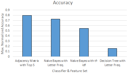
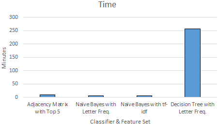
Finally, we compare all the classifiers \& feature sets that we tested in terms of their accuracy and time requirements for training and testing. We show the accuracy values that is achieved with a configuration that produces the maximum accuracy value for each classifier \& feature set combination. Figure  \ref{fig:compallacc} and \ref{fig:compalltime} show the time and accuracy results. 

 

As Figure \ref{fig:compallacc} shows, we get the highest accuracy result with our adjacency matrix model that returns the top 5 weighted values, $80\%$. It is followed by the Naive Bayes classifier with letter frequencies with $71\%$ accuracy. Then, Naive Bayes classifier with tf-idf features comes with $55\%$ accuracy. Lastly, Decision Tree with letter frequencies comes with $16\%$ accuracy. 

 

When we compare the training and testing times of the classifiers we used, Naive Bayes classifiers come as first with $5$ minutes, then our adjacency matrix model comes close with $10$ minutes, and Decision Tree is again the last one with more then $4$ hours. 

 

As having the lowest accuracy and highest training and testing time, Decision Tree is the worst model amongst the ones that we tried for our problem. Although Naive Bayes classifier with tf-idf shows relatively better performance with $55\%$ accuracy, having a better accuracy of $71\%$ of Naive Bayes classifier with letter frequencies makes it meaningless to use. As the last option we end up making a decision between Naive Bayes classifier with $71\%$ accuracy and our adjacency matrix with top 5 with $80\%$ accuracy. Naive Bayes classifier has lower accuracy but returns one single result having the highest probability. On the other hand, adjacency matrix has a higher accuracy but returns the top five results instead of one single precise result. Although it might seem as a bad thing to return top 5 results instead of one single, we believe that it is a good thing to have more than one result in the return set of the classifier. In crossword solvers, it makes a lot of sense to get an input from the user as solving a crosswords is typically an interactive activity. We believe that, instead of returning one single result and failing more with Naive Bayes classifier, using the adjacency matrix, returning the top 5 results to the user, and letting the user to decide what the word can be is more useful. Moreover, adjacency matrix has the flexibility of returning more/less than top 5 weighted words, which might provide even more inputs to the user and lets him/her select the appropriate word, and more flexibility to tune the model; whereas Naive Bayes model is fixed and restricts the possible results to only one option. Therefore, due to the domain-specific structure of our learning problem, we decided to our adjacency matrix model.

 

 

 

\section{Other approaches}

 

This section describes some other approaches that we explored. These are alternatives to the decisions that have been discarded because of practical issues or time constraints.

 

In particular here we describe an alternative to weighted category adjacency matrix described in \ref{sect:featureset1} and an interesting implementation based on a paper.

 

\subsection{WordNet similarity matrix}

 

\href{https://wordnet.princeton.edu}{WordNet} is a lexical database for the English language, it acts as both a dictionary and a thesaurus.

\href{http://www.nltk.org/}{NLTK} provides a python interface to access the WordNet corpus and his lexical resources. An interesting feature is the possibility to compute the similarity between words using different algorithms like the Path Similarity, the Leacock-Chodorow Similarity and the Wu-Palmer Similarity.

 

Because these algorithms compute the similarity between two words We thought that we could try to apply them between the labeled word and the words of its definition. So instead of using the weighted categories we associate a similarity score to each definition word. For example if the stemmed definition of "cat" is let's say {domestic, animal} we compute the similarity between "cat" and "domestic" and "cat" and "animal". These scores can then be used for the feature vector of the labeled word "cat".

 

So we found interesting to try to do that to make some comparison. We decided to use the Path Similarity as the scores are between 0 and 1. The first issue was to find a java or scala interface to have access at these methods.

We found \href{http://sujitpal.blogspot.ch/2014/04/nltk-like-wordnet-interface-in-scala.html}{here} such an interface that translates the NLTK wordnet methods in scala. Next we present briefly the Path Similarity algorithm and the reasons of why we actually did not use this matrix.

 

\subsubsection{Path Similarity}

 

This algorithm computes the semantic relatedness of words by counting nodes along the shortest path between senses in the 'is-a' hierarchies of WordNet. The score is the inverse of the distance. The score between the same two words is 1. The hierarchy is based on hypernym/hyponym trees. An hyponym is a word whose semantic field is included within that of another word, its hypernym. For example "canine" is an hypernym of "dog" and "dog" is an hyponym of "canine".

 

\subsubsection{Considerations}

 

We spend a lot of time trying to use this interface in spark because of technical issues. A problem was that these algorithms compute the similarity between only between words of the same category (Noun, Verb, Adjective, Adverb), so it's not possible to get a score similarity between a noun and an adjective because they belong to different trees. This was the major limitation.

Because of this and because of technical problems and time constraints we did not succeed to really test this approach.

 

\subsection{Reverse dictionary}

 

While exploring different alternatives of how to find a word given its definition, we found an interesting paper: \textit{Building a Scalable Database-Driven Reverse Dictionary} \cite{revDicPaper}.

 

Basically the reverse dictionary is based on five DB tables that map the words to their definitions, synonyms, hypernyms/hyponyms, similar words and the words whose definition contains such word. It then applies algorithms to find the most probable words matching an input definition.

The paper shows very good experimental results in term of scalability, performance and quality.

 

When we discovered that our project was already in an advanced stage and so, because of the big technicals efforts that such an implementation would require, we decided to continue on our direction. This way we had the opportunity to investigate our methods in a more challenging way.