Data and Analysis

We begin during the semester to test our first prototype with dextran samples. It allows us to try the prototype particularly to know if it can detect different level of fluorescence. We took pictures of different dextran dilution's samples and analysed them.

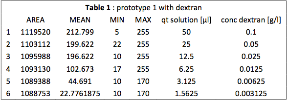
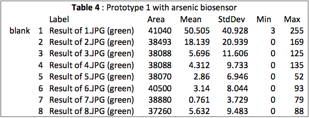
This table is an output from ImageJ. We see that the MEAN for samples 1 to 3 is really close to the MAX. We observe also a break between the third and fourth mean. This is more visible on Fig. 1.

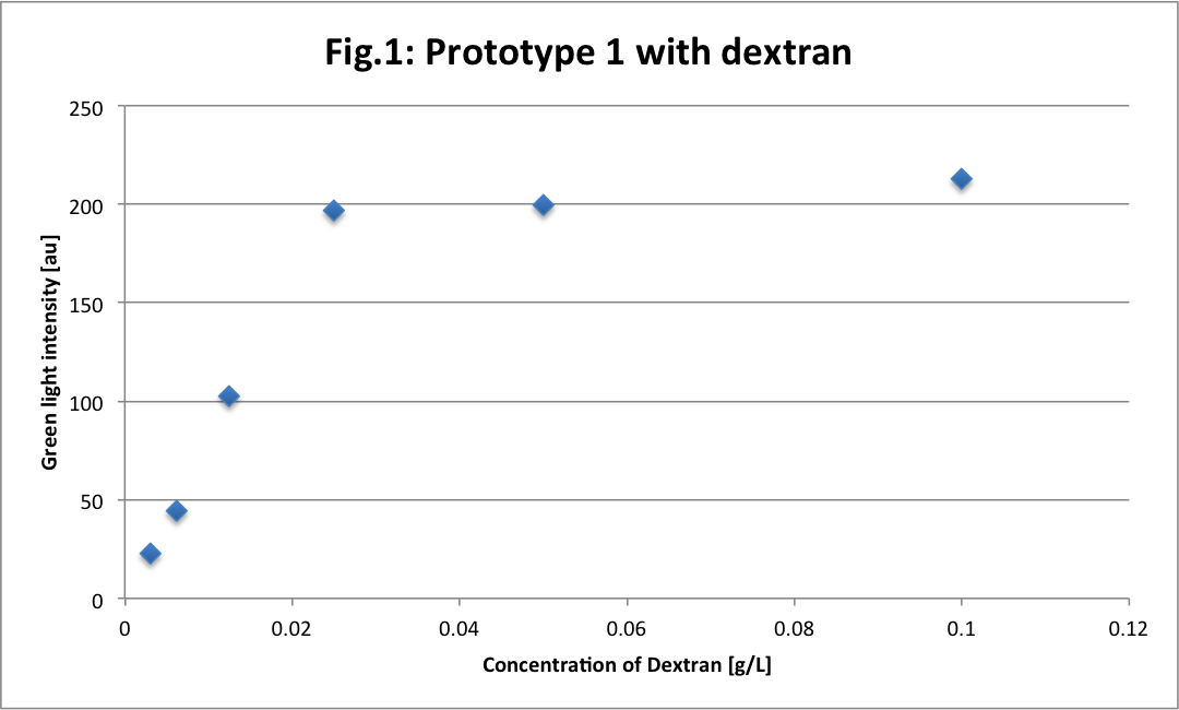
We see a clear difference between high and low concentrations because the sensibility of the camera photoreceptor is limited. When samples are too concentrated, they emit a too big intensity of green light that burns the picture. In this case, there are too much saturated pixels (value = 255 in Table 1) and they predominate on the picture. It gives a linear function according to the concentration.

This is different with small concentrations. The average of green light intensity is more “real“ and gives another linear function with concentration, because the camera could really sense and quantify the light intensity.

 

Some weeks later we received strain of eGFP bacteria from Dr. Jan Van der Meer Lab. So first we made some control measurements with a fluorometer. We expect to see an increase of fluorescence related to the decrease of dilution as well as excitation and emission peaks at 488 nm and 509 nm respectively.

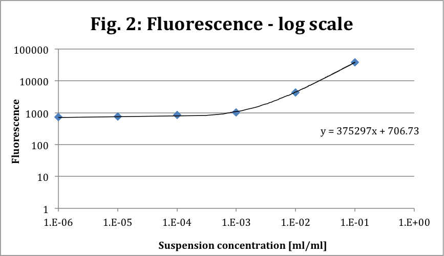
This is the fluorescence in function of the dilution for excitation at 488 nm and emission at 525 nm (log scale). The function (y) is linear as expected.

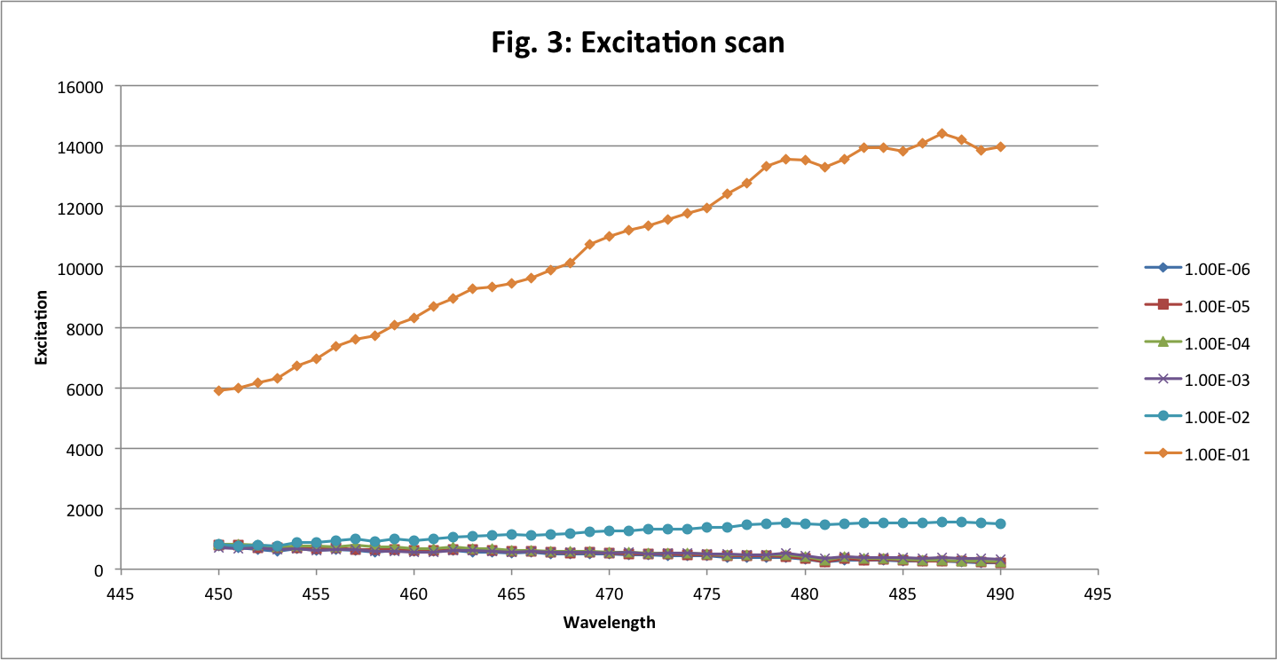
The excitation scan is from 450 to 490 nm and the emission is fixed at 525 nm.

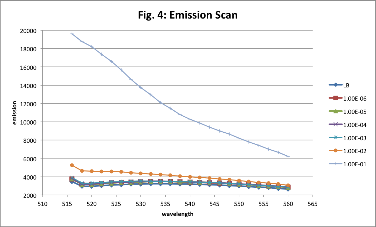
In the Fig.4 the emission scan goes from 490 to 560 nm and the excitation is fixed at 488 nm (in fact between 490 and 515 nm we get overlapping so these data are useless).

For excitation and emission wavelengths, we see that the maximum values are at 488 nm and around 509 nm as expected. The first dilution is the only significant one. The others are too small to be readable.

These measurements show that the bacteria are indeed expressing eGFP and also that fluorescence is dependent of the concentration.

Then we want to use our first device. We made a serial dilution. We plated a part of each dilution in order to count them and test samples in our prototype. We expect to see a rise of light intensity according to a drop of dilution like the first experimentation with the dextran.

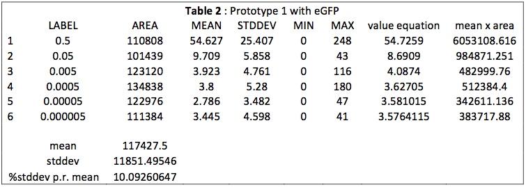
After 10^-3 the results are the same so it shows us a detection limit at 10^-3.

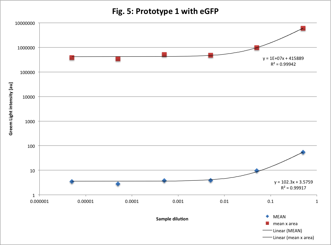
Here both are linear function (but also in log scale) as expected. The second curve (mean x area) is more precise because area change slightly between each measure so the mean is balanced by area. But it is almost the same curve. These graphs confirm the detection limit at 10^-3.

We got plates back after a growing time. We used the more diluted sample plate to be able to count the colonies. We used ImageJ in order to make it.

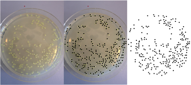
Here is the last dilution (5 x 10^-6) in process to be analysed.

After image processing we have only the spots remained. The program counted 259 colonies.

We know that we have a volume of 200µl diluted 200’000 times. So we have 259/200 ≈1.3 bacteria per µl. We multiply per 200'000 and obtain 259'000 bacteria/µl. This is the concentration after the cell culture. We know that the limit for our prototype is at 5x10^-3 thus the minimal amount of bacteria needed to be detected is 1300 bacteria per µl.

We try the second prototype with dextran like the first one for calibration. We obtain really good results.

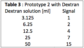
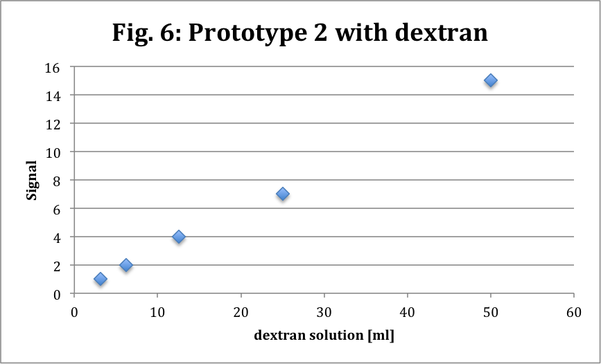
So we see a nice linear curve that confirm the increase of signal according to the concentration. We know that dextran has a greater light intensity than eGFP (about 4 times) and here the signal is very small so it has to be more difficult with eGFP.

 

Finally we use the arsenic biosensor to reach the first aim of our prototypes. We accomplish that in Van der Meer lab. First we also made a control measurement. We use a preconceived protocol to prepare the biosensor with the help of Lab’s people. Once the biosensor ready we mix it with different concentration of arsenite (ASIII) then incubate them for 2-3 hours.

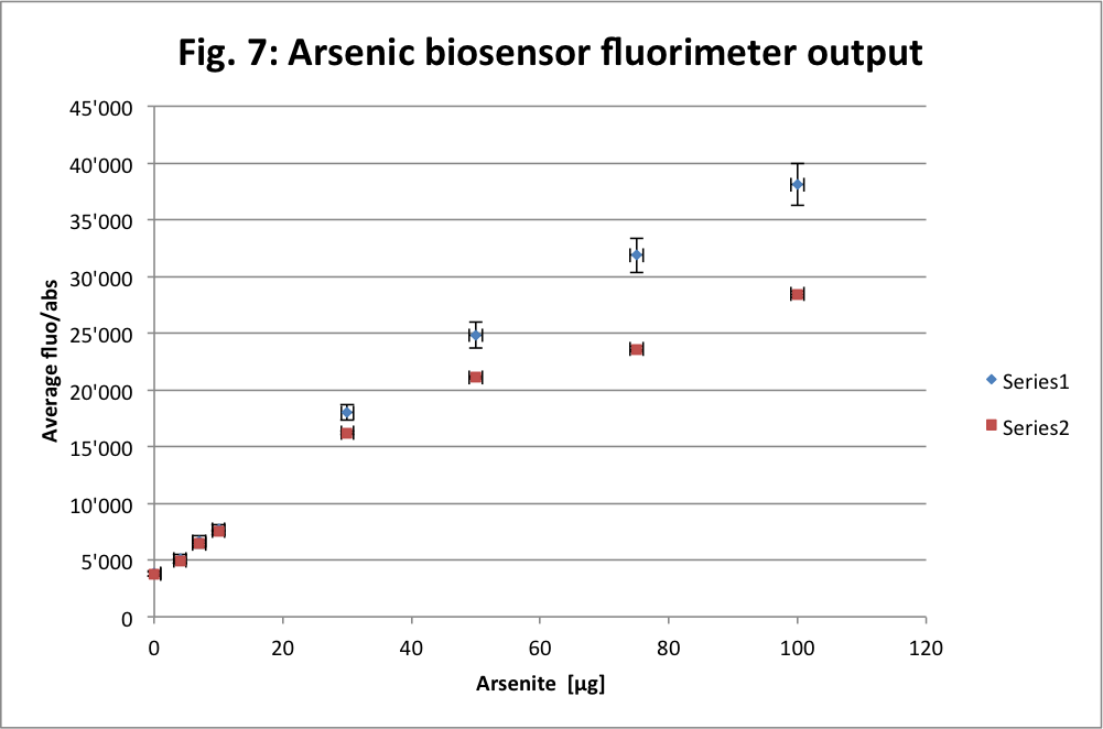
The unit used here is “the relative fluorescence units (RFU) of the induced samples divided by that of the untreated sample (background fluorescence) after hours incubation.“ as it is said in the protocol. The blue series is in an exponential phase and thus bacteria are fully active. While the red one is in a stationary phase. This is why the blue one is more linear and thus more fluorescent than the red curve.

We also brought some contaminated water samples from Martigny that we knew roughly the range (between 10 to 40 [µg/L]). But the results show less than 0 µg for each sample. After discusion we have learnt that a protocol exists to take arsenic samples and keep them without precipitate arsenic. Thus there was no enought arsenic in solution after one week.

Then we also made a test with our first prototype. Here are the results.

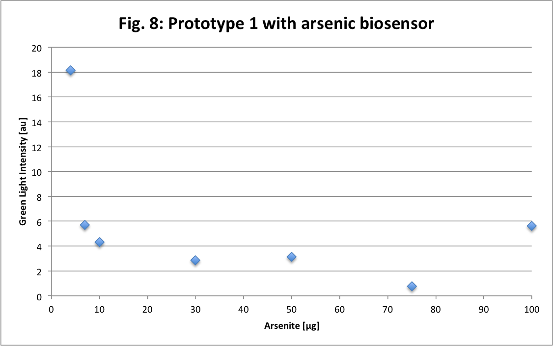
Compare to the dextran or the eGFP Figures this one is not distinct at all. We does not observe a linear curve as expected or as the Fig.7. We had some trouble during the experiment. So it might be this trouble the cause of our fail or our prototype cannot simply measure as precisely as we want.

The second prototype has no interesting results. Because the signal cannot be distinguish from the LED light despite the filter.