Coupling between cell cycle and circadian clock : Arnold tongues

Model

Deterministic model, theta is the phase of the cell cycle. Omega is the angular frequency of the circadian clock :

$latex \displaystyle{ \Large \mathrm{d}\theta/\mathrm{d}t=\omega+K\sin(\Omega t-\theta)\left(\frac{\cos(\theta)+1}{2}\right)^{n} }$ 

Stochastic case : 

$latex \displaystyle{ \Large \mathrm{d}\theta_{t}=\omega\mathrm{d}t+K\sin(\phi_{t}-\theta_{t})\left(\frac{\cos(\theta_{t})+1}{2}\right)^{n}\mathrm{d}t+\sigma_{\theta}~\mathrm{d}W_{t}}$

$latex \displaystyle{ \Large \mathrm{d}\phi_{t}=\Omega\mathrm{d}t+\sigma_{\phi}\mathrm{d}W_{t}}$

where $latex \displaystyle{ \Large W_{t} }$ are independent Wiener processes. 

Measure of frequency 

We define the measured angular frequency of a solution $latex \displaystyle{ \Large \theta(t) }$ as : $latex \displaystyle{ \Large \omega_{m}=\lim_{t\to\infty}~\theta(t)/t }$

Then for solution of the type $latex \displaystyle{ \Large \theta(t)=\omega t+f(t) }$ with $latex \displaystyle{ \Large \lim_{t\to\infty}f(t)<\infty}$, $latex \displaystyle{ \Large\omega_{m}=\omega}$.

In the stochastic case for solutions of an uncoupled oscillator $latex \displaystyle{ \Large \mathrm{d}\theta_{t}=\omega\mathrm{d}t+\sigma_{\theta}\mathrm{d}W_{t} }$ :

$latex \displaystyle{ \Large \theta_{t}\sim\ \mathcal{N}(\omega t,~\sigma_{\theta}^{2}t) }$

$latex \displaystyle{ \Large \theta_{t}/t\sim\ \mathcal{N}(\omega,~\sigma_{\theta}^{2}/t) }$

$latex \displaystyle{ \Large \omega_{m}\sim\ \mathcal{N}(\omega,0)=\omega }$

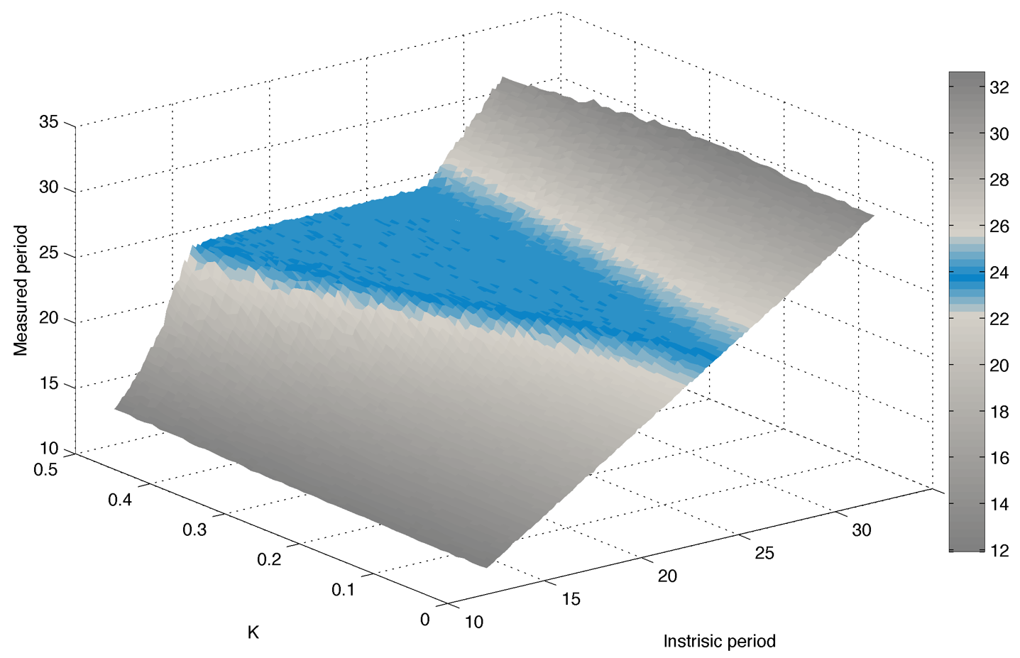
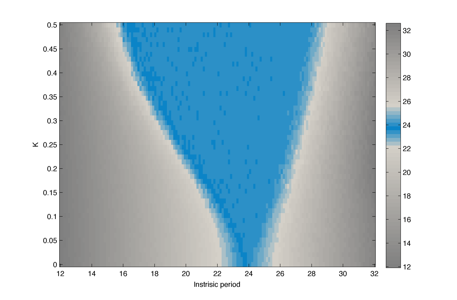
Result in the deterministic case :

Fixing the value of the noise term 

A way to fix the value of noise parameter $latex \displaystyle{ \Large \sigma_{\theta}}$ is to look at the first passage time distribution of the uncoupled oscillator $latex \displaystyle{ \Large \mathrm{d}\theta_{t}=\omega\mathrm{d}t+\sigma_{\theta}\mathrm{d}W_{t} }$ :

$latex \displaystyle{ \Large  H=\inf\{t>0\;\colon\;\theta_{t}=2\pi\}}$

Theses first passage time follow an inverse gaussian distribution (Folks and Chhikara (1978)) :

$latex \displaystyle{ \Large  f_{H}(H)=\left[\frac{2\pi^{2}\sigma_{\theta}^{-2}}{2\pi H^{3}}\right]^{1/2}\exp\left(-2\pi^{2}\sigma_{\theta}^{-2}(H-T)^{2}/(2\; T^{2}H)\right) }$

Where $latex \displaystyle{ \Large T=2\pi/\omega }$

The variance of this distribution is given by : $latex \displaystyle{ \Large \textrm{Var}(H)=\frac{\sigma_{\theta}^{2}T^{3}}{2\pi^{2}}=\frac{\sigma_{\theta}^{2}2\pi}{\omega^{3}} }$

Then $latex \displaystyle{ \Large \sigma_{\theta}=\frac{\textrm{Std}(H)\;\omega^{3/2}}{\sqrt{2\pi}} }$

From Yeom et al. (2010) we can estimate $latex \displaystyle{ \Large \textrm{Std}(H)=1\;[hour] }$ for both circadian and cell cycle, the circadian angular velocity Omega is $latex \displaystyle{ \Large 2\pi/24\;[rad/hour]}$ and the cell cycle angular velocity $latex \displaystyle{ \Large \omega=2\pi/T}$ with $latex \displaystyle{ \Large T\in[12,\:32] }$

Result :

Simulating experimental conditions 

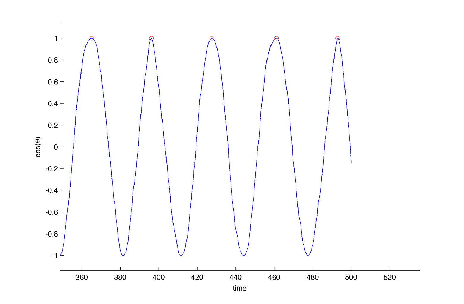
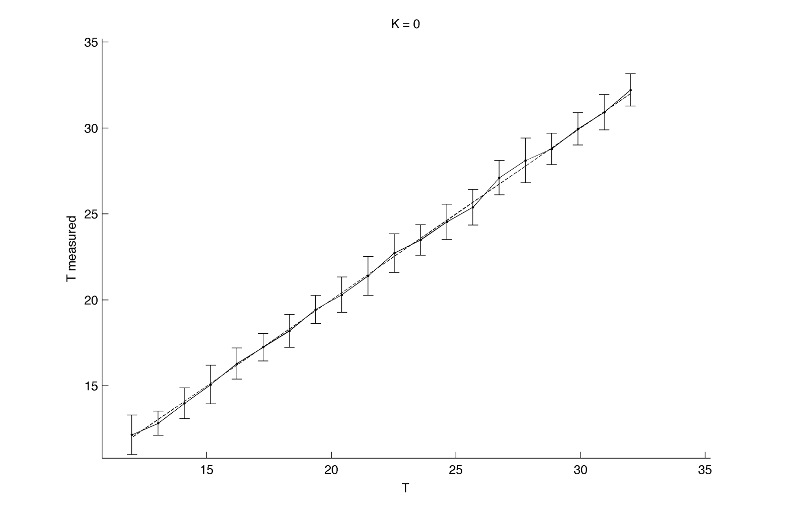
In practice we cannot neither measure $latex \displaystyle{ \Large \omega_m }$ nor fix the coupling strength K. A more realistic measure is to look at the peak-to-peak distance for different realisations (cells).

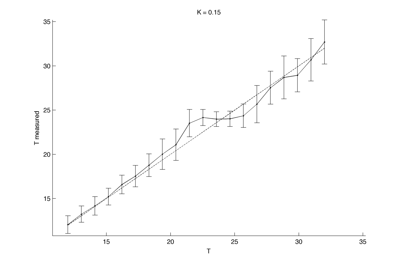
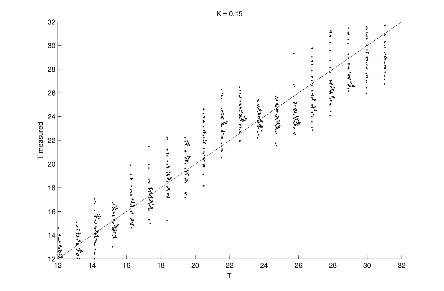
Here we assume we are able to measure only one period per cell, for 40 cell per intrinsic frequency, and 20 intrinsic frequency are tested. We fix K at 0.15 :

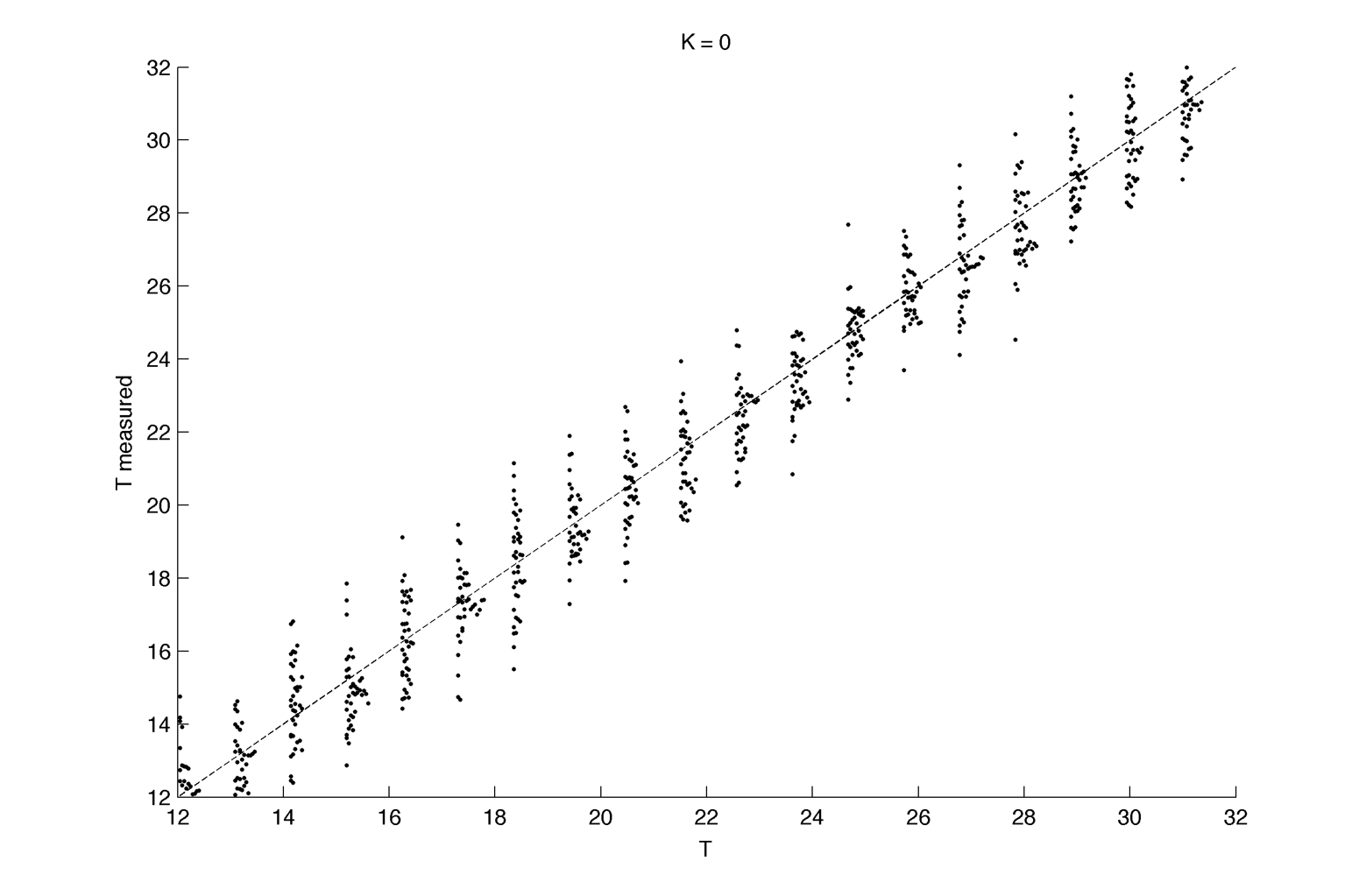
The same for K = 0 (cells without circadian rhythms) :

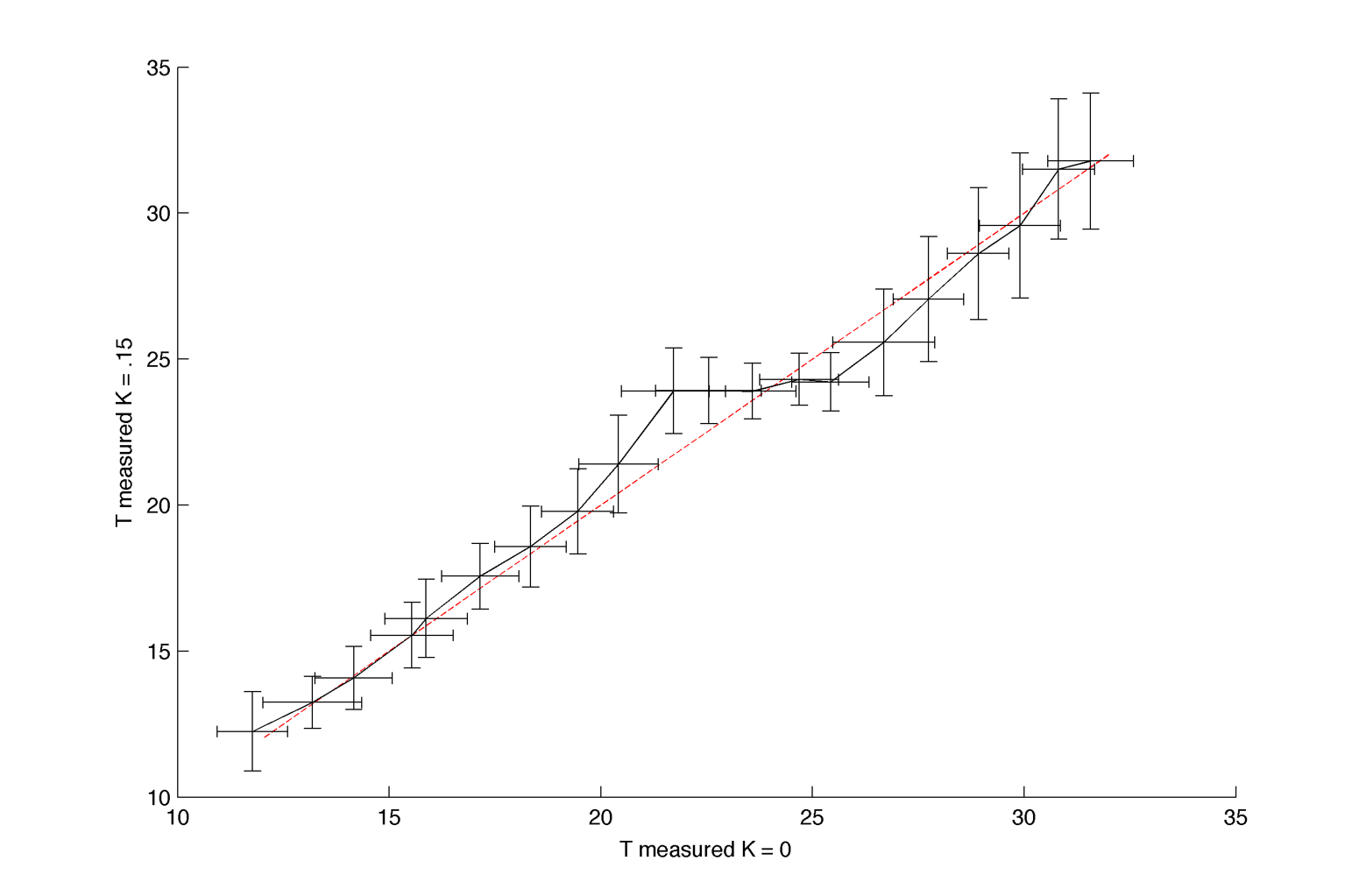
As we don't know the instrinsic period T we should do something like that (or use the temperature as a proxy) :

Distribution plot :