Arnold tongues - additional information

Navigation

• Home
• Sitemap

This wiki

This page

Arnold tongues

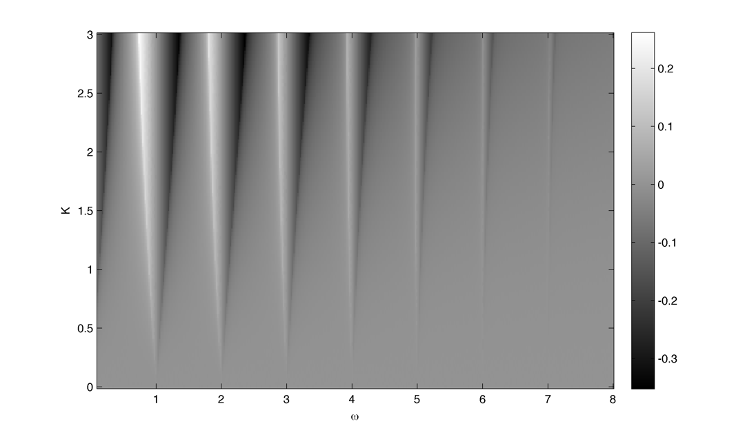
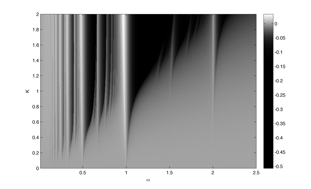
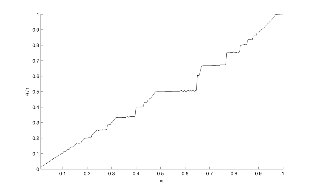
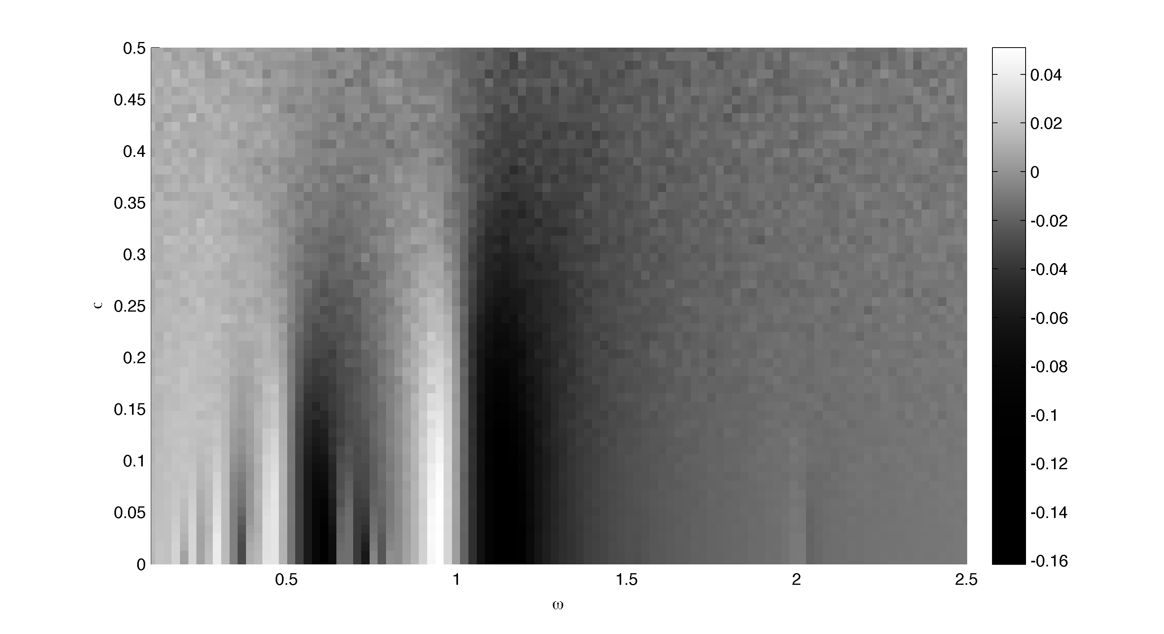
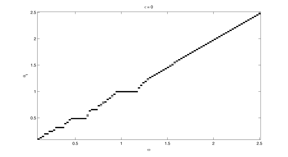
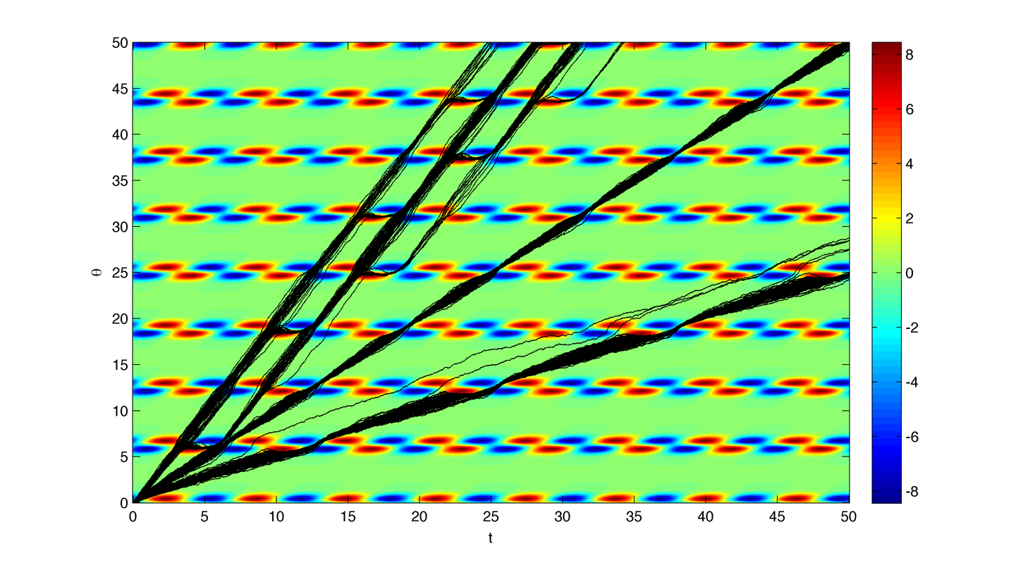
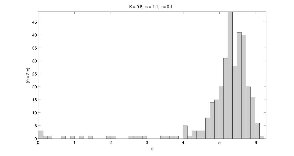
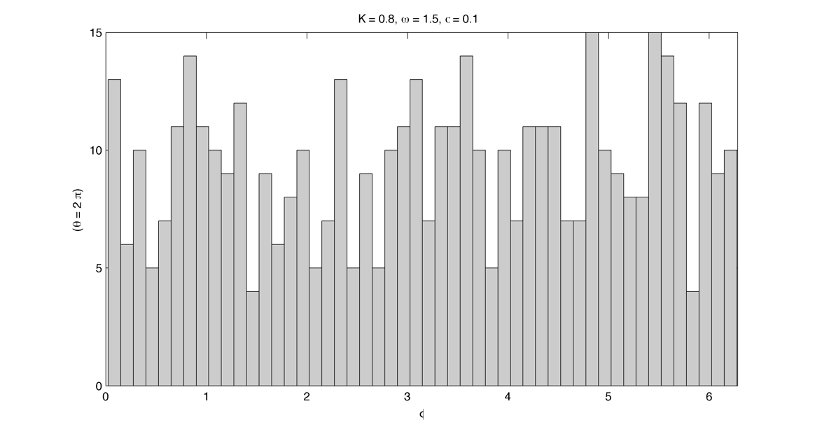
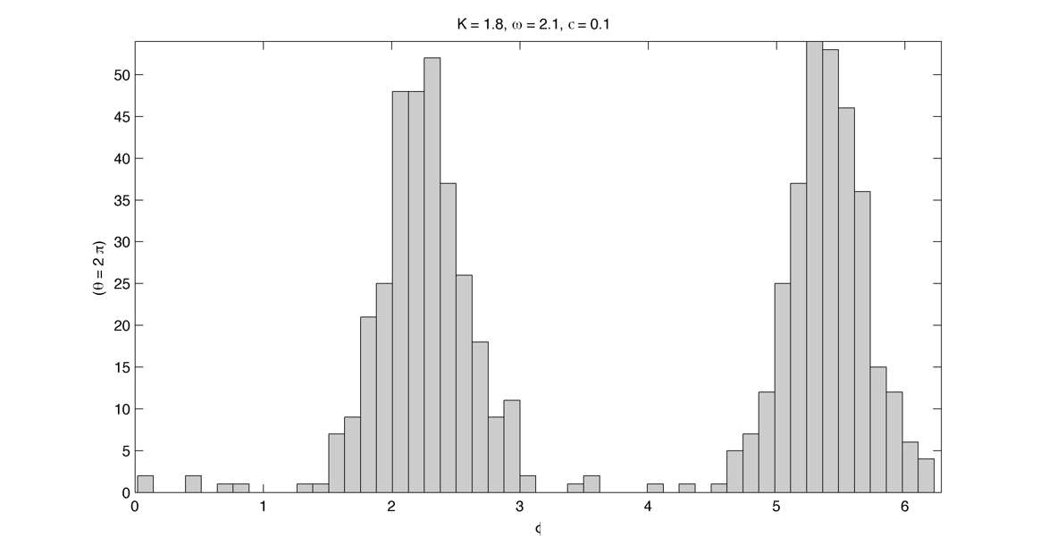
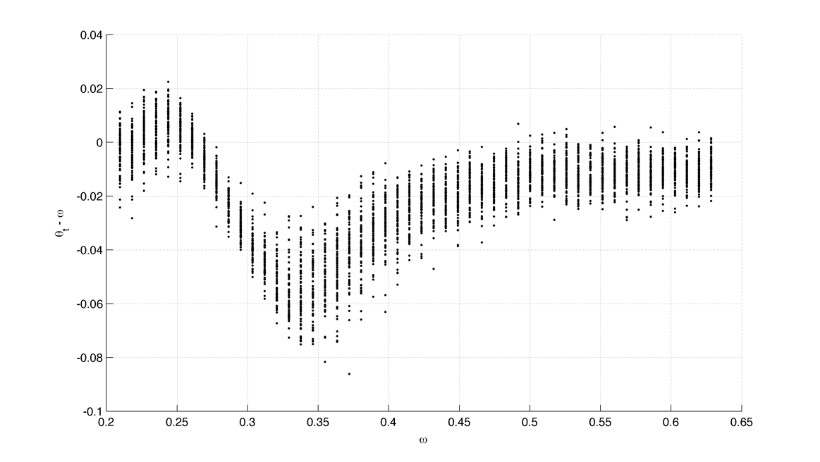
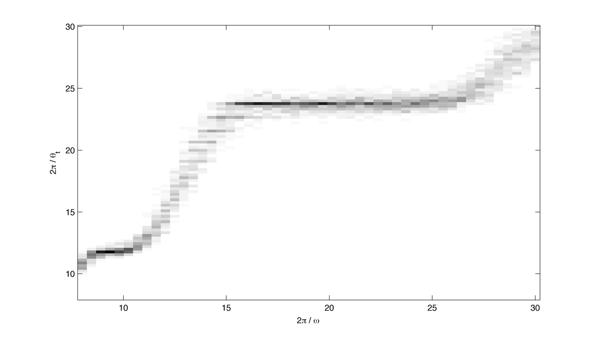
Compute the arnold tongues for different type of oscillator.

$\displaystyle{\Large }$

Measure of effective angular frequency ?

$\displaystyle{ \Large \omega_m = lim_{t \to\infty} ~ \theta(t) / t }$

If $\displaystyle{ \Large \theta(t) = \omega t + \phi + f(t) }$ with $\displaystyle{ \Large lim_{t \to\infty} ~ | f(t) | < \infty }$ then $\displaystyle{ \Large \omega_m = \omega}$ .

If we have periodic cumulative slippage with period $\displaystyle{ T_s }$ i.e. $\displaystyle{ \Large \theta(t) = \omega t + \phi + 2 \pi \lfloor t / T_s \rfloor }$ then $\displaystyle{ \Large \omega_m = \omega + 2 \pi / T_s = \omega + \omega_s}$ .

1. Continuously kicked phase oscillator

Model 1 :

$\displaystyle{ \Large \theta_t = \omega + K \sin(\theta) \left ( \frac{ \cos(\Omega ~ t) + 1} {2}\right ) ^ n }$ (1)

Here is $\displaystyle{ \Large lim_{t \to\infty} ~ \theta(t) / t - \omega }$ in the $\displaystyle{ (\omega, K) }$ plane with n = 20 :

n = 200 :

2. Continuously kicked phase oscillator 2

Model 2:

$\displaystyle{ \Large \theta_t = \omega + K \sin(\Omega~t - \theta) \left ( \frac{ \cos(\theta) + 1} {2}\right ) ^ n }$ (2)

n = 20 :

Better plot : $\displaystyle{ \Large \frac{ \partial ( \theta(t) / t ) } {\partial \omega} }$ :

n = 200 :

Devil's Staircase :

3. Continuously kicked phase oscillator 2 stochastic :

Model 3 :

$\displaystyle{ \Large \mathrm{d}\theta_t = \omega \mathrm{d}t + K \sin(\Omega~t - \theta_t) \left ( \frac{ \cos(\theta_t) + 1} {2}\right ) ^ n \mathrm{d}t + \sigma_{\theta} ~\mathrm{d}W_t}$ (3)

$\displaystyle{ \Large \mathrm{d}\phi_t = \Omega \mathrm{d}t + \sigma_{\phi} \mathrm{d}W_t }$ (4)

Note : solution of eq. 4 :

$\displaystyle{\Large {f(\phi)}_t = \Omega ~ f_\phi + \frac{1}{2} \sigma_{\phi}^2 ~ f_{\phi \phi} }$

$\displaystyle{ \Large f(\phi, t) = \frac{1}{ \sqrt{ 2 \pi {\sigma_\phi}^2 t } } \exp \left ( - (\phi - \Omega t)^2 / ( 2 {\sigma_\phi}^2 t) \right ) }$

$\displaystyle{ \Large f(\phi | t) \sim\ \mathcal{N}(\Omega t, ~{\sigma_\phi}^2 t) }$

In this case our measure of angular frequency :

$\displaystyle{ \Large \Omega_t = ~ \phi_t / t \sim\ \mathcal{N}(\Omega, ~{\sigma_\phi}^2 / t) }$ .

We can try to find the period distribution at a given time t by making the change of variable $\displaystyle{ \Large T_t = 2\pi / \Omega_t }$ :

$\displaystyle{ \Large f(T|t)=\left[\frac{2\pi}{\sigma_{\phi}^{2}t^{-1}T^{4}}\right]^{1/2}\exp\left(-\frac{(2\pi/T-\Omega)^{2}}{2\sigma_{\phi}^{2}t^{-1}}\right) }$

Surprisingly evaluating at t = T it gives back the inverse gaussian distribution corresponding to the first passage time problem ( $\displaystyle{ \Large \Omega_t = 2\pi}$ ) :

$\displaystyle{ \Large f(T | t=T) = \left [ \frac{ {2 \pi}^2 {\sigma_\phi}^{-2} }{ 2 \pi T^3 } \right] ^{1/2} \exp \left ( - {2 \pi}^2 {\sigma_\phi}^{-2} (T - T_\Omega)^2 / {2 T_\Omega^2 T} \right ) }$

As t goes to infinity the distribution looks like a dirac centered on $\displaystyle{ \Large 2 \pi / \Omega }$

Here is the mean of $\displaystyle{ \Large \theta(t) / t - \omega }$ in the $\displaystyle{ (\omega, \sigma_{\theta,\phi} ) }$ plane with n = 20 and fixed K = 0.8 :

The noise seems to smooth the modes, the strongest ones (1:1, 1:2) being more robust.

Here is the stochastic devil's staircase for increase $\displaystyle{ \sigma_{\theta,\phi} }$ :

Contraction analysis could be a nice tool to study the stochastic system. Here is a plot of contracting regions (in blue), divergent region (in red) with some trajectories in black

with $\displaystyle{ \Omega = 1, \sigma_{\phi} = 0, n = 10, K = 3, \omega = 2, 1, 0.5}$ :

In the green zone, where the coupling is not active, the trajectories diffuse and drift freely. In the slower modes $\displaystyle{\omega < \Omega}$ this "free" time is longer.

In the (1:1) case the phase variance as the trajectories touch the contracting zone get reduced and the same process start again.

In the (2:1) case ( $\displaystyle{\omega = 2, ~\Omega = 1}$ ) the trajectories hit an divergent region each two period which lead to a lot of "phase slippage" (always in the same direction).

In the (1:2) case ( $\displaystyle{\omega = 1/2, ~\Omega = 1}$ ) the trajectories always pass through a contracting region, but as the "free time" is longer there is some slippage.

We can also compute the distribution of "mitosis" $\displaystyle{ ( \theta = 2\pi + 2 k \pi ) }$ along "circadian phase" $\displaystyle{ ( \phi ~ mod ~ 2\pi ) }$ , it can

be unimodal (1:1), uniform (phase drifting) or multimodal (2:1) :

More realistic parameters :

Problems : we would like to take $\displaystyle{ \Omega = 2\pi / 24 }$ (circadian period of 24 hour) and vary $\displaystyle{ \omega }$ in a realistic range. We would like to fix the noise variance to have a realistic period variability but:

1. Stochastic period is not really well defined

2. We need cell cycle and circadian rhythm period variability data. (does it scale with temperature ?)

Here is the distribution of angular frequencies for K=0.4, n=40 and 80 samples per intrinsic frequencie for "realistic" parameters :

The same for the period T :

The same but for K = 1.5 :