|
Navigation
 This wiki
This page This wiki
This page
|
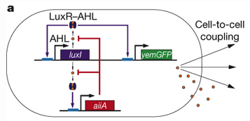
A synchronized quorum of genetic clocks
Data :
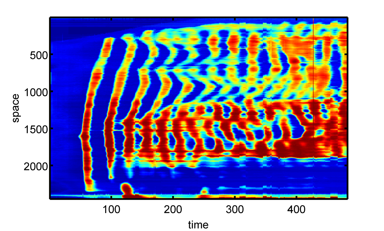
Boundary condition seems to be zero concentration on each side as waves vanish on the boundary.
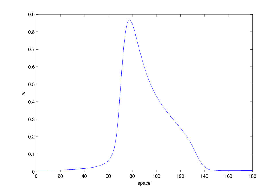
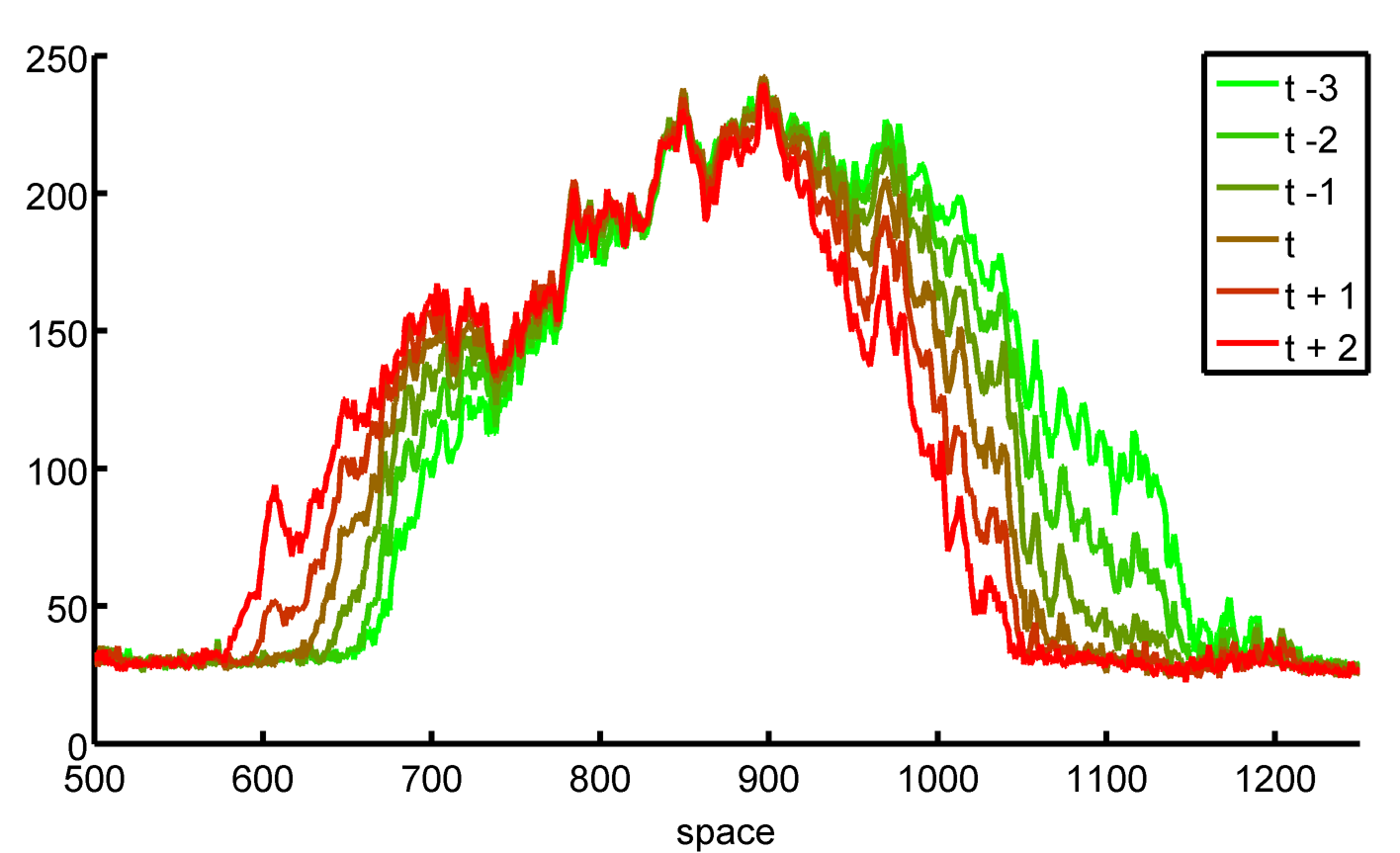
Wave form in space :
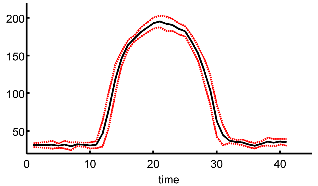
Oscillation in time :
Looks symmetric.
Excitable model III : $latex \displaystyle{ \Large w_t = \alpha_w \frac{w^2}{1 + w^2} - \gamma_{vw} ~ v \frac{w}{k + w} - \lambda_w ~w + I}$ $latex \displaystyle{ \Large v_t = \frac{w^2}{1 + w^2} - v}$
p = 90 400 3 5
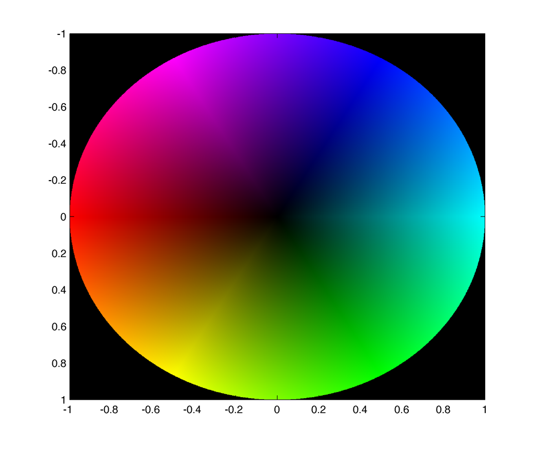
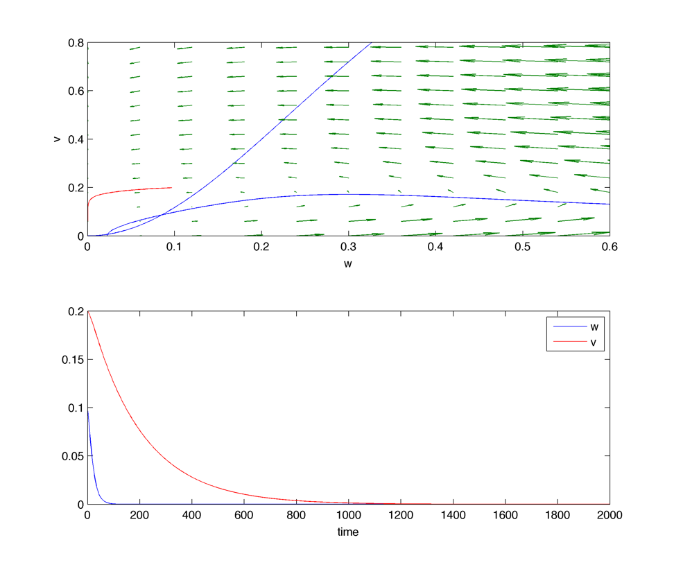
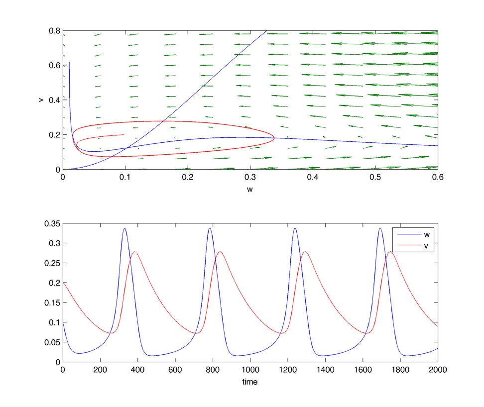
Phase portrait (vector field is plotted in HSV), the hopf bifurcation occurs when the two isoclines meet at the inflexion point of the w one :
Colormap :
Bifurcation diagram :
Higher repression :
Addition of A : $latex \displaystyle{ \Large w_t = \alpha_w \frac{w^2}{1 + w^2} - \gamma_{vw} ~ v \frac{w}{k + w} - \lambda_w ~w + A}$ $latex \displaystyle{ \Large v_t = \frac{w^2}{1 + w^2} - v}$ $latex \displaystyle{ \Large A_t = \alpha_A w - \lambda_A~ A} ~~~ (\lambda_A = 0.5)$
Making the change of variable z = x -ct in the diffusion coupled system :
$latex \displaystyle{ \Large -c \dot{w} = \alpha_w \frac{w^2}{1 + w^2} - \gamma_{vw} ~ v \frac{w}{k + w} - \lambda_w ~w + A}$ $latex \displaystyle{ \Large -c \dot{v} = \frac{w^2}{1 + w^2} - v}$ $latex \displaystyle{ \Large -c \dot{A} = \alpha_A w - \lambda_A ~A + D \ddot{A}}$
Or : $latex \displaystyle{ \Large \dot{w} = -1/c \alpha_w \frac{w^2}{1 + w^2} + 1/c \gamma_{vw} ~ v \frac{w}{k + w} + 1/c \lambda_w ~w -1/c A}$ $latex \displaystyle{ \Large \dot{v} = -1/c \frac{w^2}{1 + w^2} + 1/c v}$ $latex \displaystyle{ \Large \dot{A} = B}$ $latex \displaystyle{ \Large D \dot{B} = -\alpha_A w + \lambda_A ~A - c~B }$
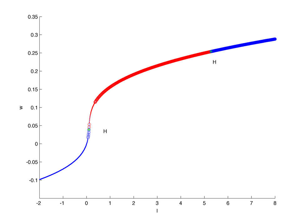
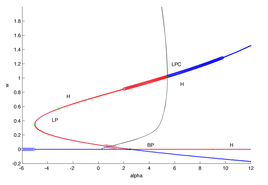
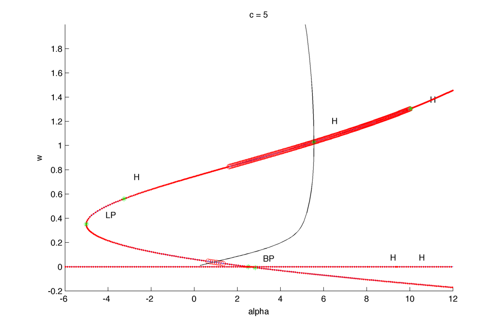
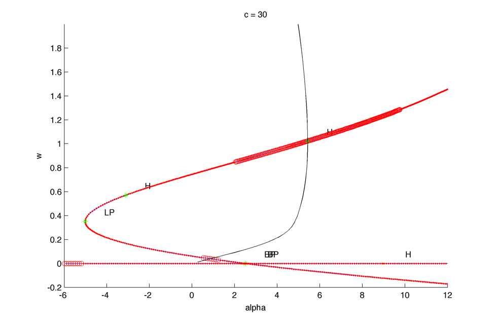
Bifurcation diagram for two different speed (position of the Hopf bifurcation change a bit) :
The same but for different set of parameters :
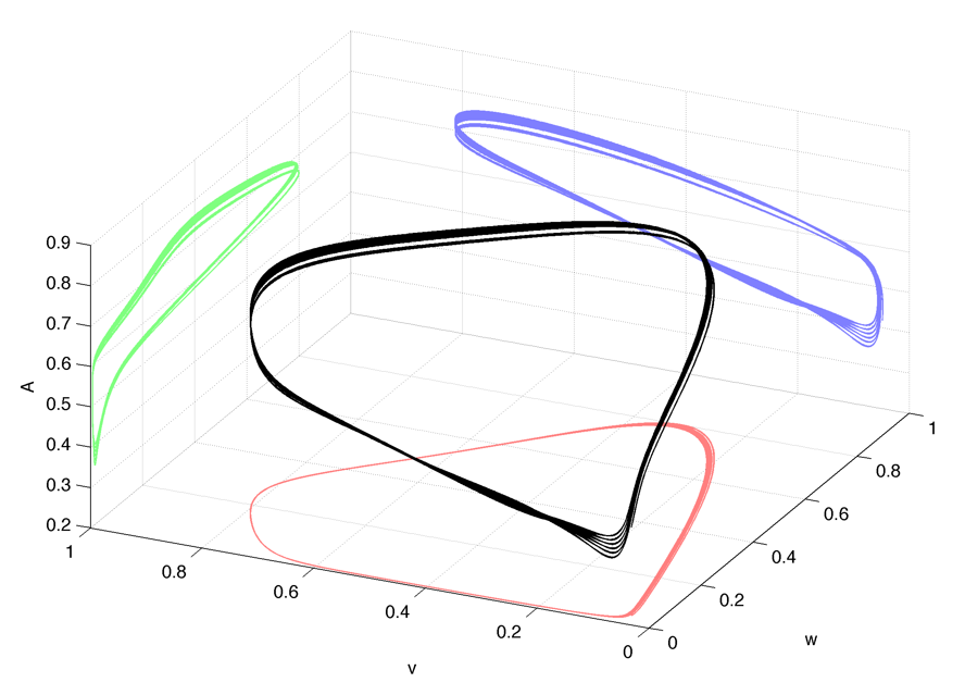
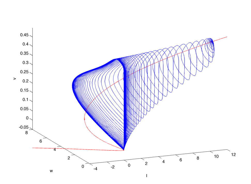
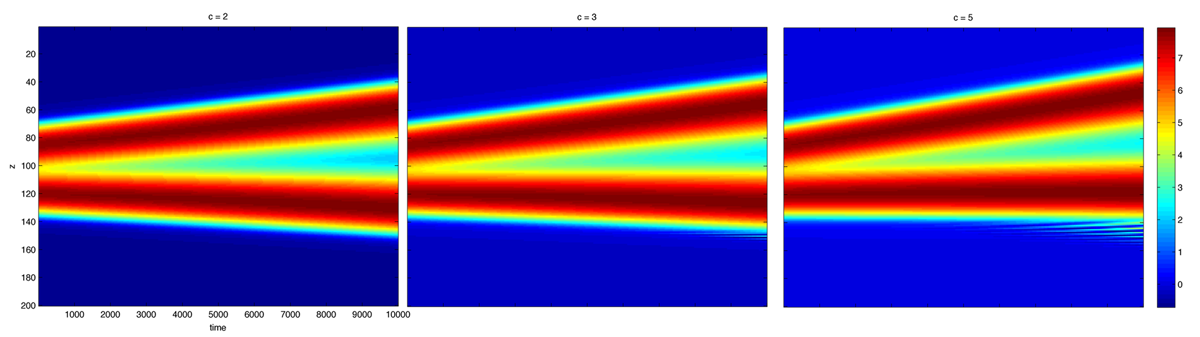
Simulation of the system using coordinate change $latex \displaystyle{ (z,t) = (x-ct, t) }$ and for different speed c (alpha = 4) :
It seem we have a stationary solution for c around 5 (measured speed from simulations is 5.4). Here is an animation of the limit cycle for different speed with the orbit from the simulation of the system in the (x,t) plane.
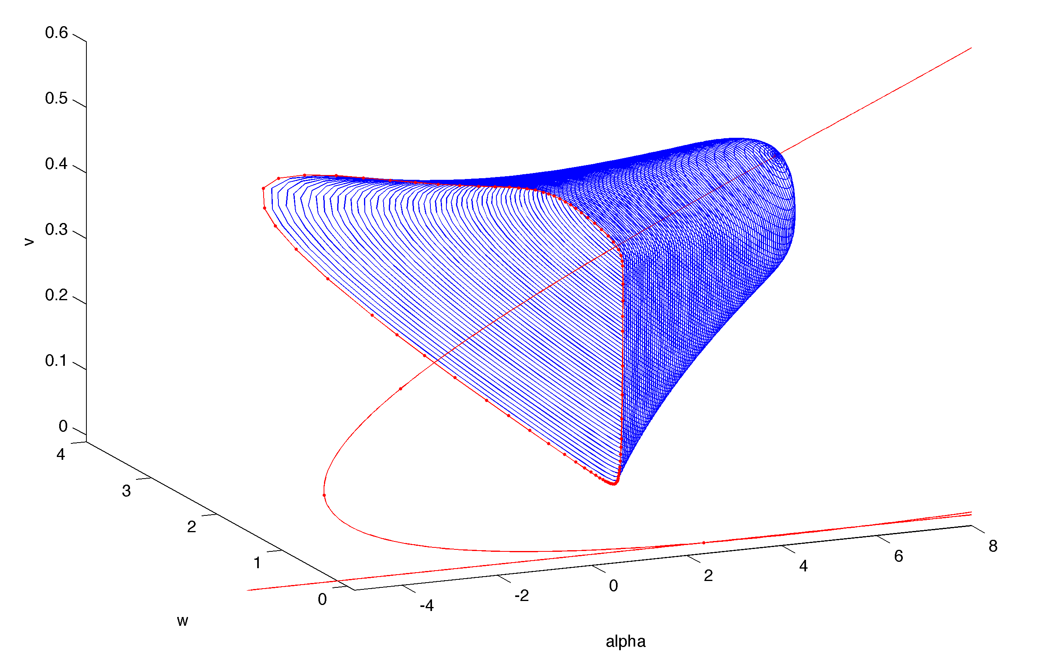
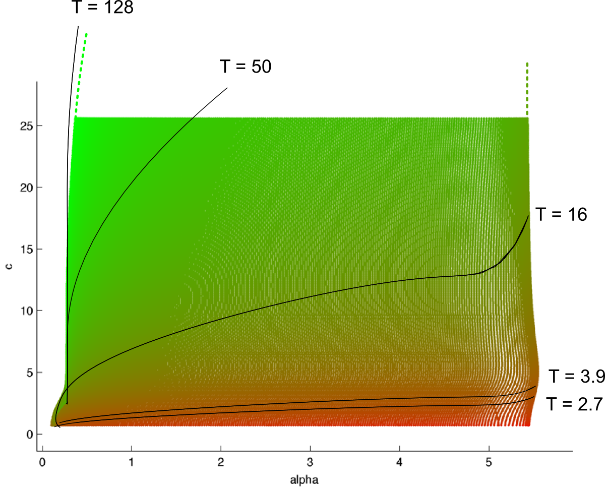
Limit cycle with period (T) in the (alpha,c) plane :
Excitable model :
$latex \displaystyle{ \Large w_t = \alpha_w \frac{w^2}{k_w^2 + w^2} - \gamma_{vw} ~ w \frac{v }{k_{vw} + v} - \lambda_w ~w + I}$ $latex \displaystyle{ \Large v_t = \alpha_v \frac{w^2}{k_v^2 + w^2} - \lambda_v ~v}$
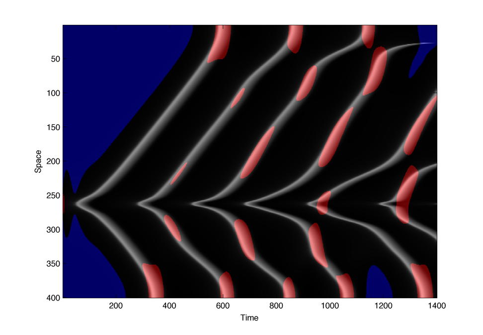
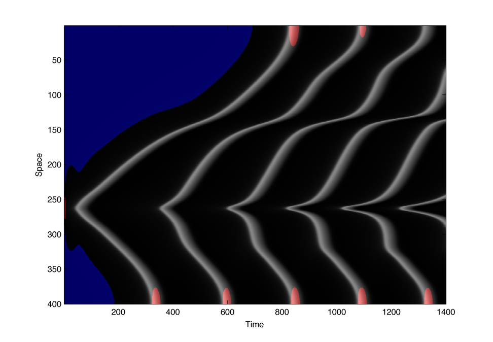
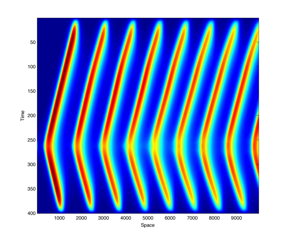
w in space time with red indicating regions above the hopf bifurcarion (A > 0.8) and blue region in the stable region (A < 0.2) :
Theses parameters gives a nice result :
Gamma : 3.00 Alpha : 12.00 D : 8.00 rep : 200.00 a1 : 0.30 a2 : 0.80 g1 : 10.00 g2 : 5.00 wprod : 60.00 vprod : 10.00 Length : 10.00 Nx : 400.0 Dx : 0.025 Dt : 0.00003 Nt : 200000.0 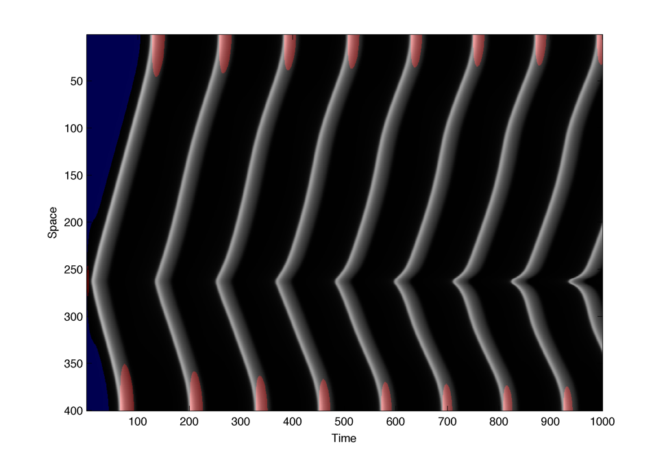 But the front shape does not look symmetric :
  Theses waves trains should correspond to a limit cycle in the transformed system below but it seems difficult to analyse...
Excitable model 2: $latex \displaystyle{ \Large w_t = \alpha_w \frac{w^2}{k_w^2 + w^2} - \gamma_{vw} ~ w \frac{v^2}{k_{vw}^2 + v^2} - \lambda_w ~w + I}$ $latex \displaystyle{ \Large v_t = \alpha_v \frac{w^2}{k_v^2 + w^2} - \lambda_v ~v}$
I = 0 :
I = 2 :
Replacing input I by a diffusion agent A :
$latex \displaystyle{ \Large w_t = \alpha_w \frac{w^2}{k_w^2 + w^2} - \gamma_{vw} ~ w \frac{v^2}{k_{vw}^2 + v^2} - \lambda_w ~w + \alpha_{Aw}~A(x,t)}$ $latex \displaystyle{ \Large v_t = \alpha_v \frac{w^2}{k_v^2 + w^2} - \lambda_v ~v}$ $latex \displaystyle{ \Large A_t = \alpha_A w - \lambda_A ~A + D A_{xx}}$
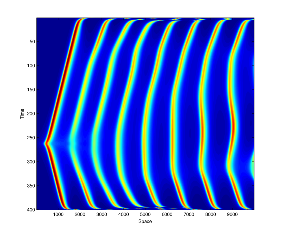
A(x,t) :
Problems : repressor and activator have the same promoter, so $latex \displaystyle{ \Large k_w^2 = k_v^2 }$. Degradation term seems a bit complicated, this simpler model shows the same behavior : $latex \displaystyle{ \Large w_t = \alpha_w \frac{w^2}{k^2 + w^2} - \gamma_{vw} ~ w ~ v - \lambda_w ~w + \alpha_{Aw}~A(x,t)}$ $latex \displaystyle{ \Large v_t = \alpha_v \frac{w^2}{k^2 + w^2} - \lambda_v ~v}$ $latex \displaystyle{ \Large A_t = \alpha_A w - \lambda_A ~A + D A_{xx}}$
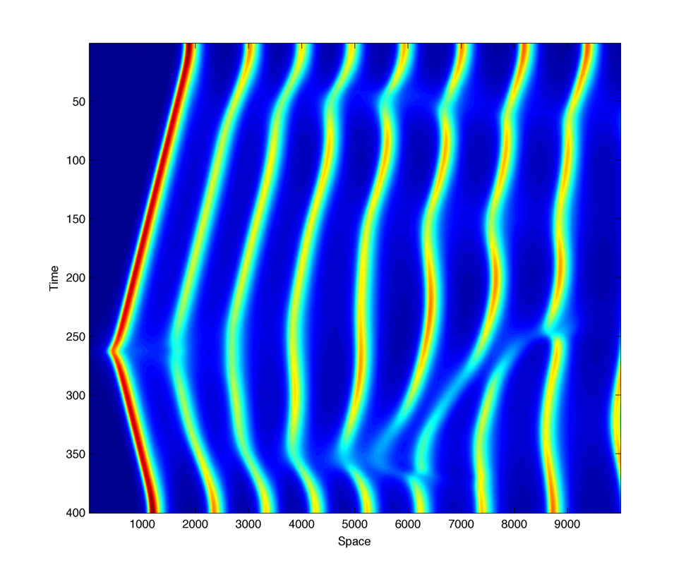
Also the GFP reporter doesn't diffuse out of the cells so we should plot w instead of A, but the boundary behavior is quite strange :
With zero derivative :
There is waves moving in opposite direction but the start from a given distance from the boundary and not from the boundary an seen in the data.
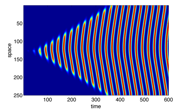
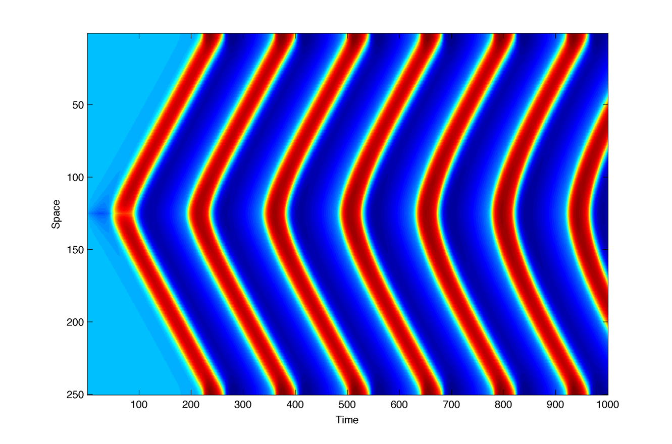
Simulation with coupled oscillators :
Gamma : 50.00 Alpha : 800.00 D : 0.40 Omega : 35.00 (0.00) Mu : -0.10 Length : 10.00 Nx : 250.00 Dx : 0.040 Dt : 0.0001
Here oscillators were initialized to zero except for some in the middle. In the data, the first oscillation travel the all space, but in the simulation the oscillations slowly build up in space. It seem it is not possible to change this while keeping the delay of ~one period between the middle and the end of an oscillation front.
It seem that a FitzHugh-Nagumo model should be more adapted :
|
Share |


