Add diffusion on each specie to make the stability easier 

Making the change of variable z = x -ct in the diffusion coupled system :

$\displaystyle{ \Large  -c \dot{w} = \alpha_w  \frac{w^2}{1 + w^2}  - \gamma_{vw} ~ v  \frac{w}{k + w} - \lambda_w ~w  + A + \epsilon \ddot{w}}$ 

$\displaystyle{ \Large  -c \dot{v} =  \frac{w^2}{1 + w^2}    - v  + \epsilon \ddot{v}}$  

$\displaystyle{ \Large  -c \dot{A} = \alpha_A  w    - \lambda_A ~A + D \ddot{A}}$ 

Or :

$\displaystyle{ \Large   \dot{w} = W}$

$\displaystyle{ \Large   \dot{v} = V}$

$\displaystyle{ \Large   \dot{A} = B }$ 

$\displaystyle{ \Large   \dot{W} = 1/\epsilon ( - \alpha_w  \frac{w^2}{1 + w^2}  + \gamma_{vw} ~ v  \frac{w}{k + w} +  \lambda_w ~w  - A - c W )}$

$\displaystyle{ \Large   \dot{V} = 1/\epsilon(  -\frac{w^2}{1 + w^2}    +  v - c V )}$  

$\displaystyle{ \Large   \dot{B} =  1/ D ( -\alpha_A  w    + \lambda_A ~A - c~B  )}$   

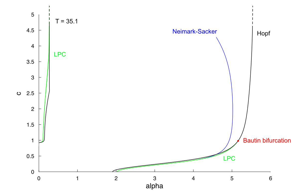
We take $\displaystyle{ \Large  \epsilon = 0.01}$.

 The bifurcation diagram look a bit different :

Period :

Amplitude of w (max - min), level set :

Stability 

Raw data 

k=0, black : unstable

k=pi / T, black : unstable

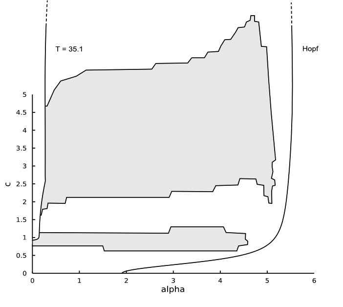
Schematic :

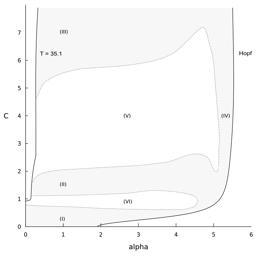
Smoothed version :

(I)

(II)

(III)

(IV)

(V) (Stable)

(VI) (Stable)

Simulating perturbed stationary solution in the original system 

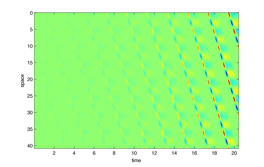
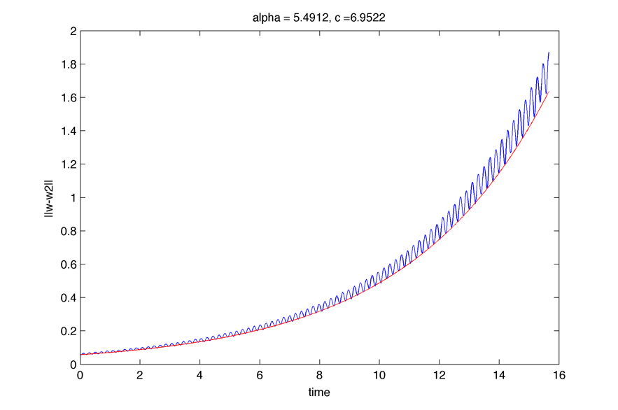
Here is a plot of the norm of the difference between stationary solution w(x,t) and perturbed solution w2(x,t), $\displaystyle{ \Large   w_2(x,0) = w(x,0) + \delta \psi(x) }$ where $\displaystyle{ \Large \psi(x) }$ is the eigenfunction associated with eigenvalue $\displaystyle{ \Large \lambda }$ :

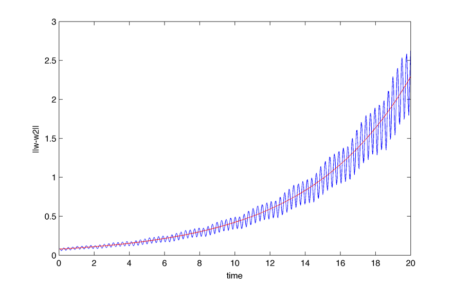
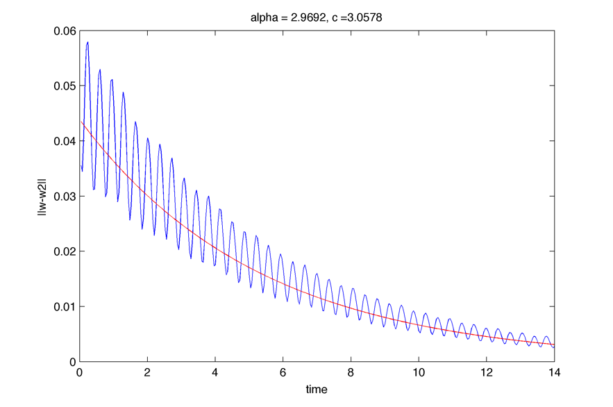
Here is the same plot integrated on space (blue), the red curve is $\displaystyle{ \Large \propto e^{\lambda t}  }$ (k = 0):

If we wait long enough we can also see the perturbation :

Negative eigenvalue (k=0):

k=pi / T :

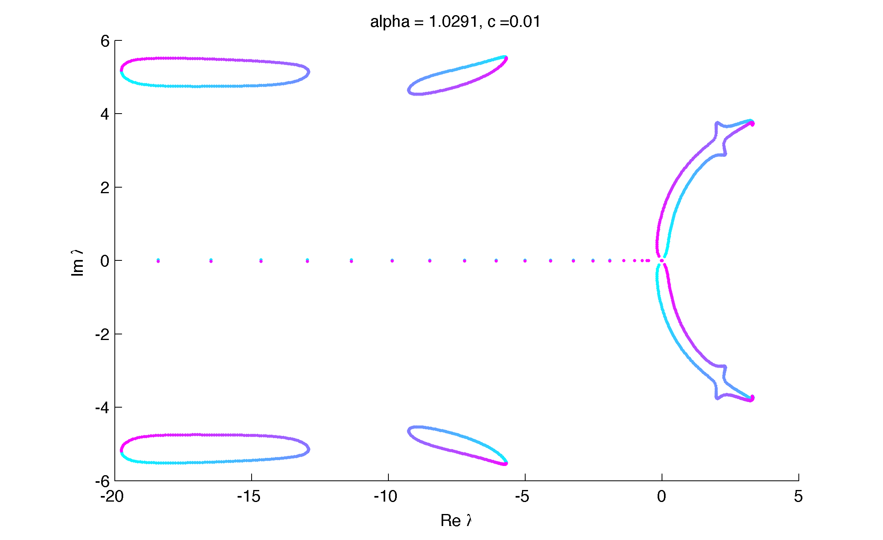
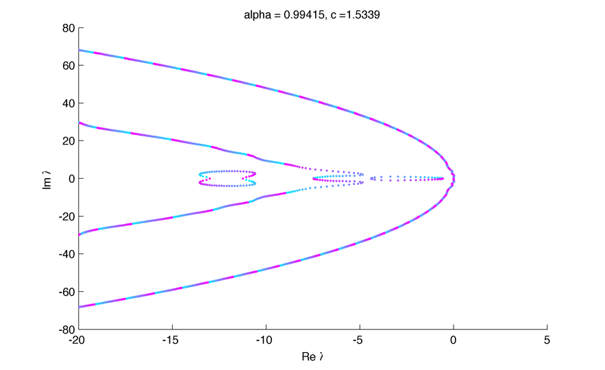
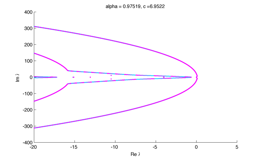
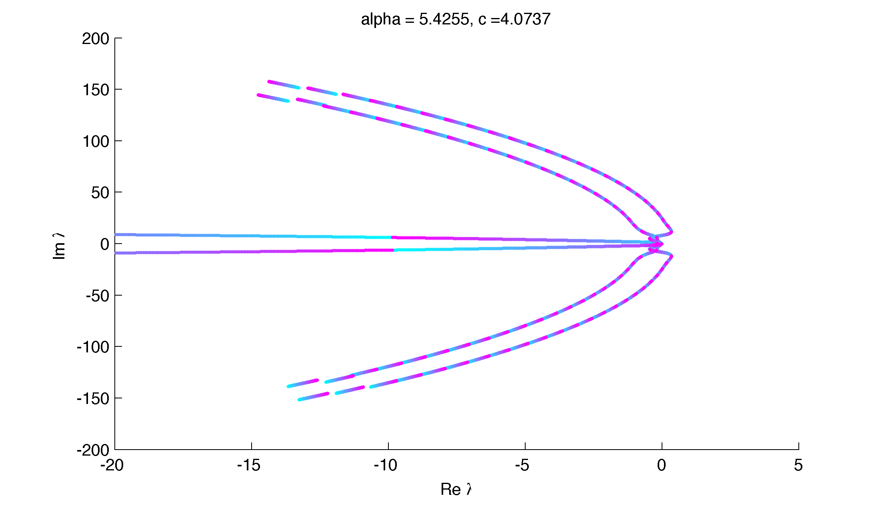
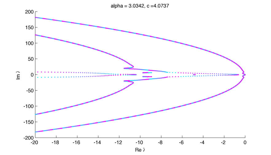
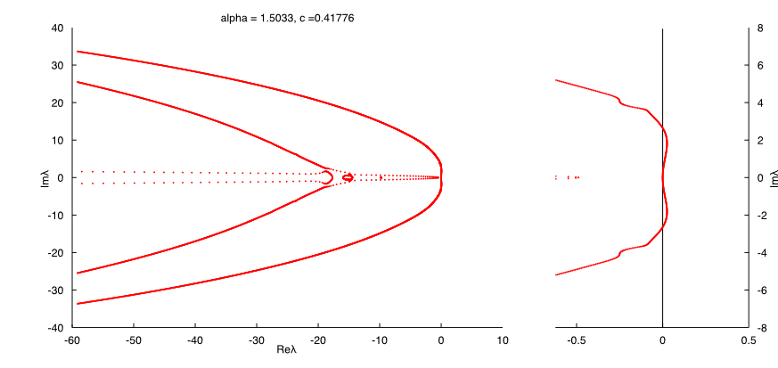
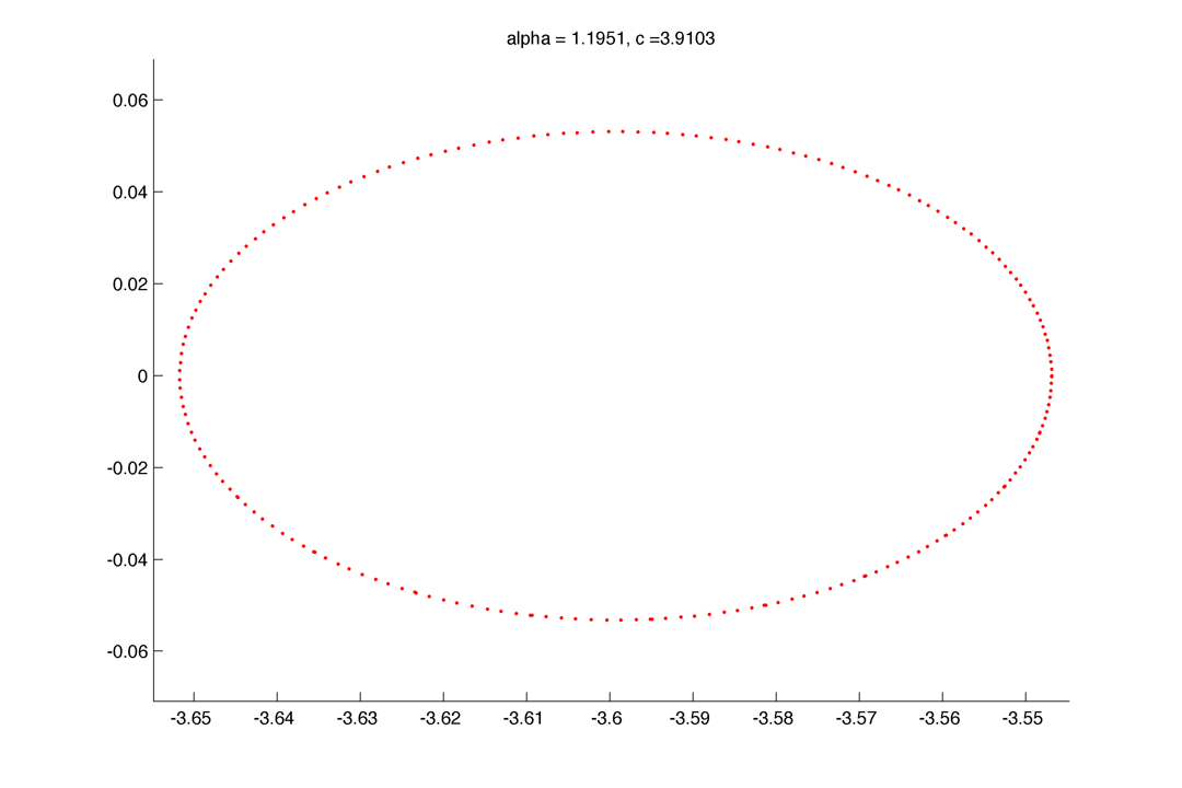
Spectrum (unstable) :

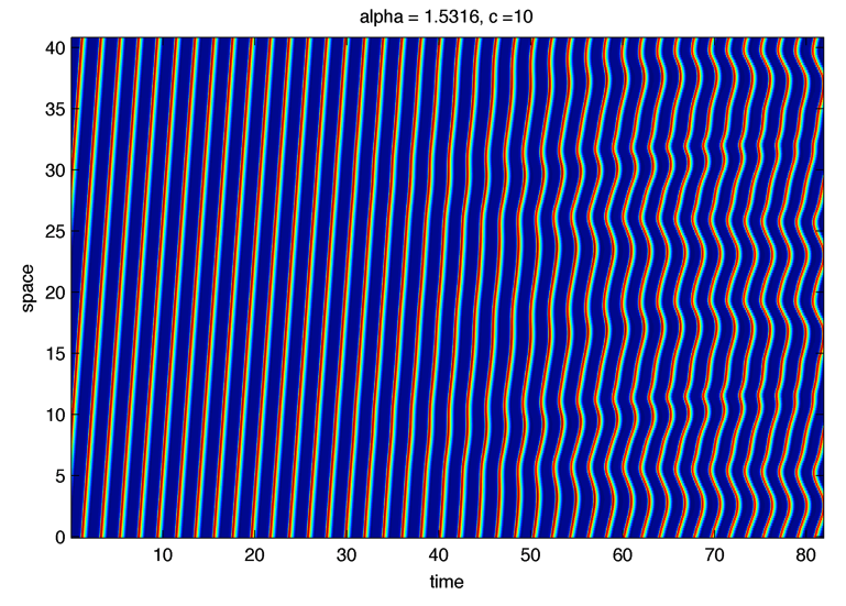
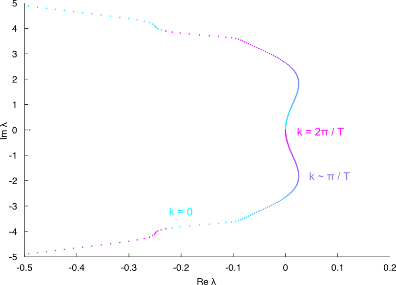
Instabilities seems to be in k = pi over T :

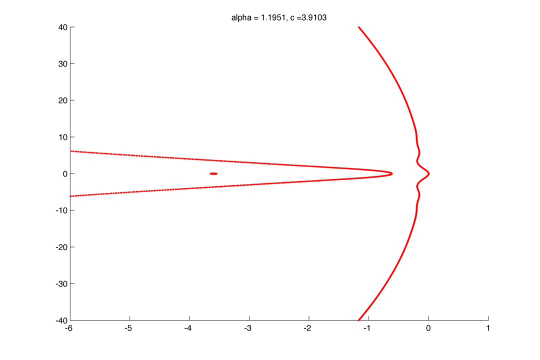
\Little circles !

The dynamic of formation of the little circles as alpha decrease :