The model :

$\displaystyle{ \Large w_t = \alpha_w \frac{w^2}{1 + w^2} - \gamma_{vw} ~ v \frac{w}{k + w} - \lambda_w ~w + A}$

$\displaystyle{ \Large v_t = \frac{w^2}{1 + w^2} - v}$

$\displaystyle{ \Large A_t = \alpha_A w - \lambda_A~ A}$

Phase portrait :

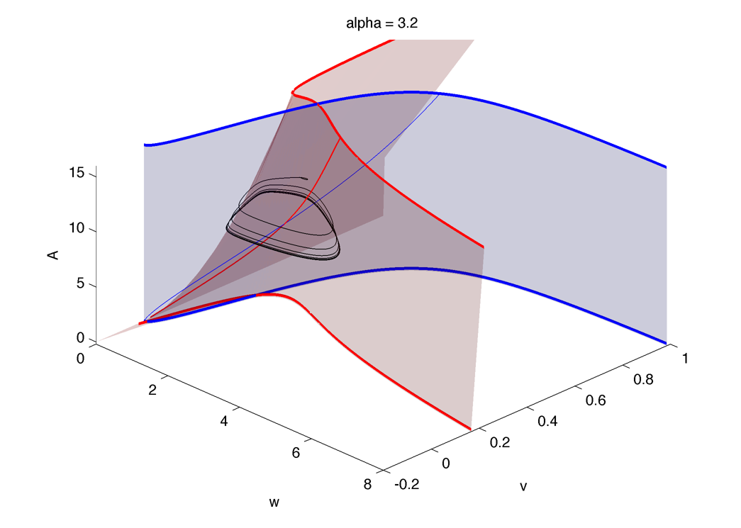
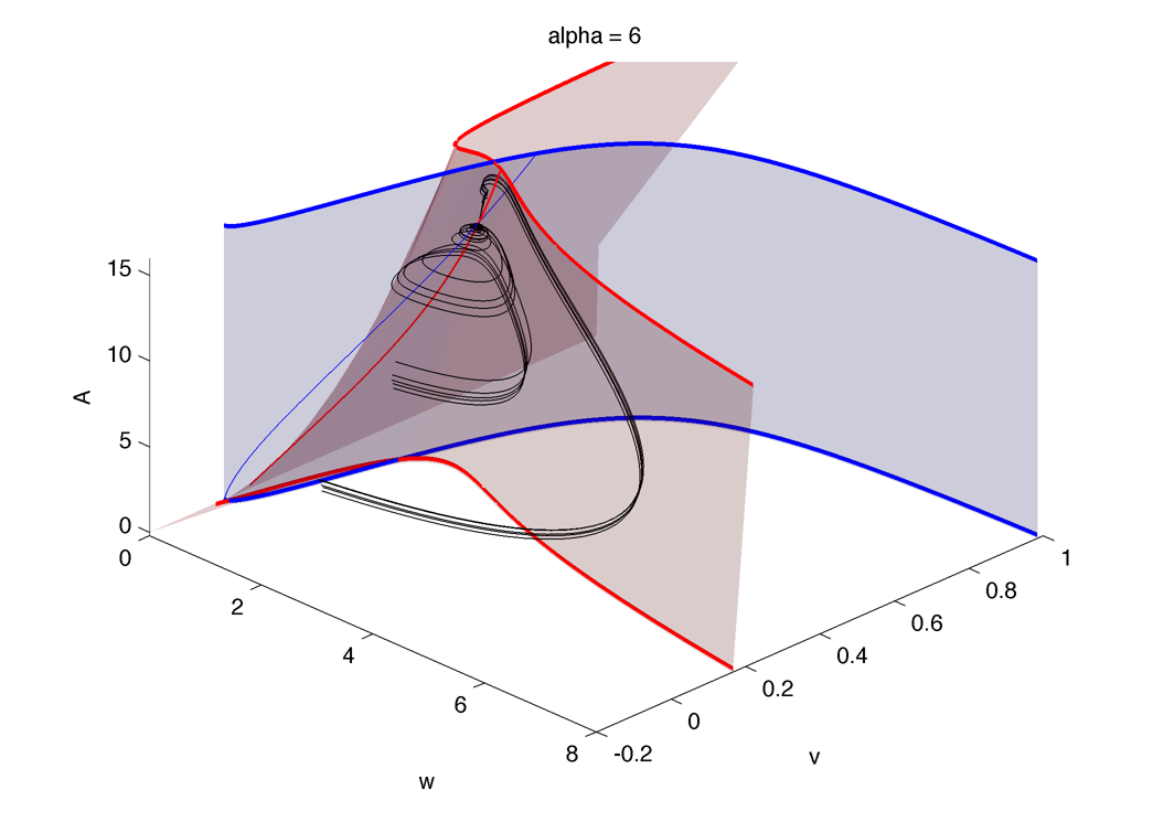
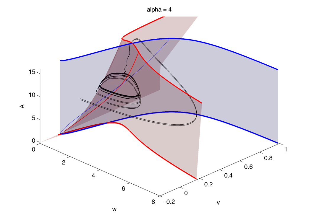
Here is projection in the (w,v) plane of the surfaces $\Large w_t = 0$ (in  red) and $\Large v_t = 0$ (blue) and a trajectory (black). The surface $\Large A_t =0$ is a is simple plane :

Which is similar to the 2D case :

The same plot but from a different view, the red curve on the red surface is $\Large w_t, A_t = 0$, and the blue $\Large v_t, A_t = 0$.

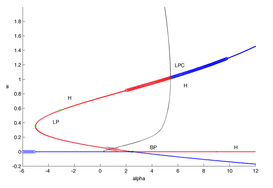
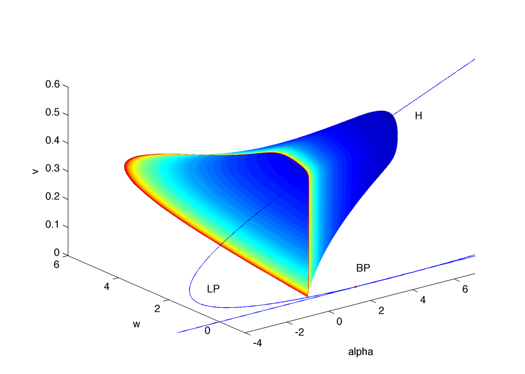
Bifurcation diagram. It seems that the limit cycle (black) in passing trough the fixed point but it doesn't, it's an effect of the projection. At alpha = 0.272 there is an LPC and the limit cycle period diverge to infinity.

Above the Hopf bifurcation the stable fixed point has two imaginary eigenvalue and a real one.

Then bellow the Hopf bifurcation the two imaginary eigenvalues become unstable :

The solutions that enter the limit cycle through the one-dimension stable manifold are the one that come from a high value of A (the 2D system has a limit cycle bellow I~=11 and and stable fixed point otherwise). Theses solutions start with low v, so that they are "kicked  out" far in w.

Then bellow the branch point there is coexistence of a limit cycle and of a stable fixed point :

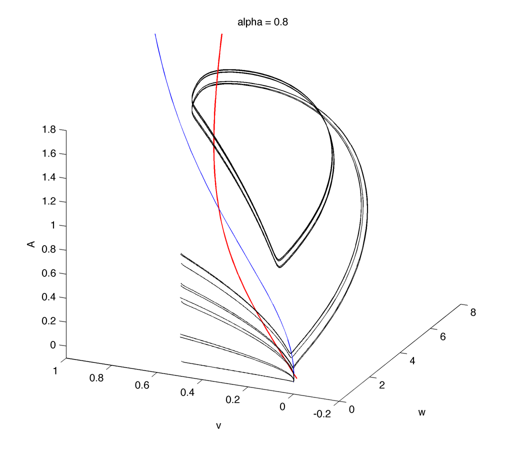
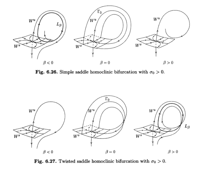
The limit cycle then disappear through a saddle homoclinic bifurcation (twisted according to Kuznetsov, p.217), here is the limit cycle with large period :

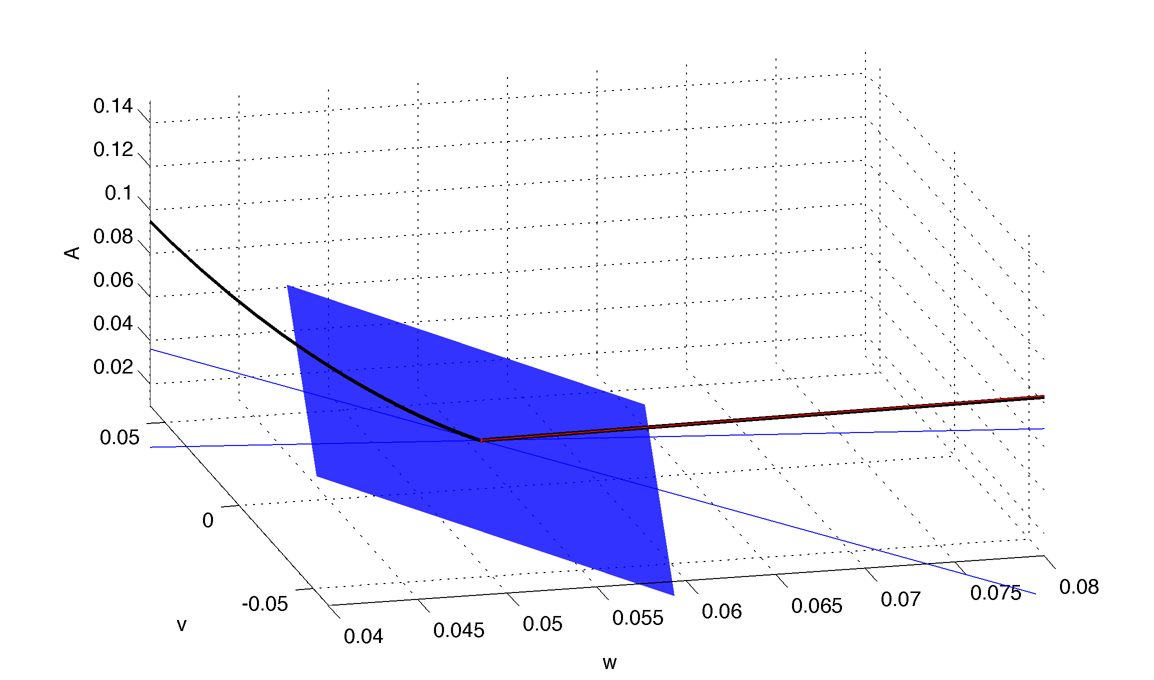
The limit cycle connects with a unstable fixed point with a two dimensional stable manifold (blue) and a one dimensional unstable one (in red) :

Difference between twisted and simple homoclinic :

Bifurcation diagram. It seems that the limit cycle (black) in passing trough the fixed point but it doesn't, it's an effect of the projection. At alpha = 0.272 there is an LPC and the limit cycle period diverge to infinity.