Perform Active Electrode Compensation

Current-clamp experiments in which the same electrode is used to stimulate and record from a neuron are biased. This bias can however be compensated using Active Electrode Compensation (Brette et. al, 2008; Badel et al. 2009).

 

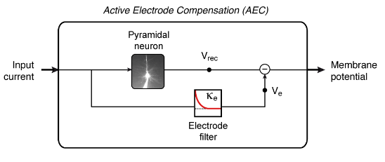
Figure: schematic representation of Active Electrode Compensation (AEC). The injected current is passed through the electrode filter (Ke). The resulting signal (Ve) approximate the time-dependent voltage-drop through the electrode and has to be subtracted from the recorded voltage (Vrec) to recover the membrane potential. Further details about AEC can be found in the original manuscript.

 

To perform Active Electrode Compensation using the methods described in the manuscript (see Figure above), create a new object myAEC of the class AEC_Badel. Later, this object will be assigned to the experiment myExp and will be used to compensate for the electrode bias.

 

from AEC_Badel import *
myAEC = AEC_Badel(myExp.dt)

The variable myExp.dt is the inverse of the experimental sampling frequency.

 

1. Define parameters

According to Equation 11 (Pozzorini et al. 2015), the optimal linear filter is expanded in rectangular basis functions. Use the function myAEC.K_opt.setMetaParameters() to define these basis functions: 

 

myAEC.K_opt.setMetaParameters(length=150.0, binsize_lb=myExp.dt, binsize_ub=2.0, slope=30.0, clamp_period=1.0)

 

The parameter length defines, in ms, the total duration of the filter. The width of the rectangular basis functions increases from binsize_lb to binsize_ub, also in ms. The parameter slope determines the speed at which the width increases. During the first clamp_period ms, the width of the basis functions is artificially clamped to binsize_lb.

 

In order to estimate the electrode filter, the tail of the optimal linear filter is fitted with a single exponential function (see Equation 14 of Pozzorini et al. 2015). To specify, in ms, the region of the optimal linear filter to which the exponential fit is performed, use the following command:

 

myAEC.p_expFitRange = [3.0,150.0]       

 

To improve accuracy, the electrode filter can be estimated several times. Specify the number of repetitions with the following command:

myAEC.p_nbRep = 15                                                                                         

 

2. Apply AEC to the experimental data

myAEC has first to be assigned to the object myExp. The function myExp.performAEC() can then be used to compensate all the voltage traces within myExp:

 

myExp.setAEC(myAEC)  
myExp.performAEC()

 

3. Detect spikes

The function myExp.detectSpikes() can be used to detect spikes. Spike times are defined as the moments where the voltage trace crosses 0.0 mV from below (first argument). To avoid multiple detections of the same spike, a period of absolute refractoriness of 4.0 ms is used (second argument).

 

myExp.detectSpikes(0.0, 4.0)  

 

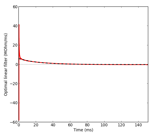
4. Visualize the optimal linear filter and the electrode filter used for AEC

To plot the optimal linear filter and the exponential function fitted on its tail, use the following function:

myAEC.plotKopt()

To plot the electrode filter used to compensate the voltage recordings, use the following command:

myAEC.plotKe()

 

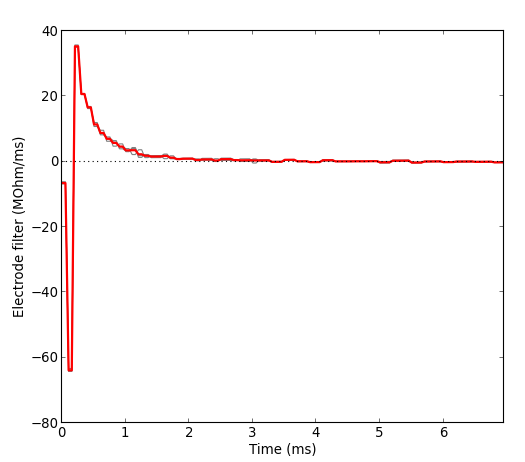
The red line shows the average filter. Gray lines indicate the results from individual repetitions.

 

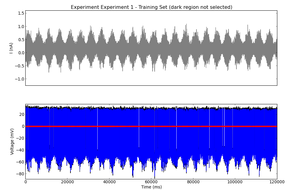
5. Plot the experimental data

By plotting the training set once again, it is now possible to visualize the results of AEC. The recorded voltage is shown in black and the membrane potential obtained after AEC in blue. Detected spikes are denoted by red circles.

myExp.plotTrainingSet()

 

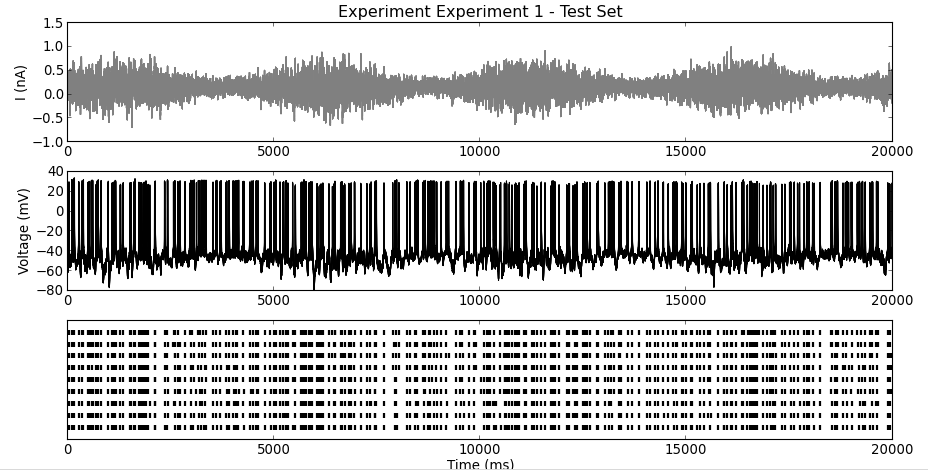
By plotting the test set it is now possible to visualize the voltage traces after AEC (middle, black) , as well as a raster plot of the spiking responses to different frozen-noise current injections (bottom, black raster).

myExp.plotTestSet()

At this stage, data have been successfully preprocessed. In the next step, this data will be used to fit a Generalized Integrate-and-Fire model.