
- français
- English
Load the experimental data
The experimental data have to be loaded using the class Experiment. You can assign a name to your experiment and specify the time step dt defining the experimental sampling frequency. The experimental data provided here have been acquired at 10 kHz, consequently the time step is dt = 0.1 ms.
from Experiment import *

  myExp = Experiment('Experiment 1', 0.1)
According to our protocol (see Figure), an experiment consists of several current-clamp injections:
- a subthreshold AEC injection used for Active Electrode Compensation
- a training set injection used for GIF model parameter extraction
- several test set (frozen-noise) injections used to assess the model performance
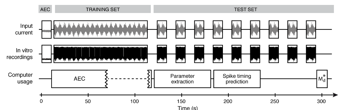
Figure: schematic representation of the experimental protocol. AEC stands for Active Electrode Compensation, a computational methods introduced by Brette et. al. 2008 and Badel et al. 2009 for data preprocessing . Md* is a spike-train similarity measure introduced by Naud et al. 2011 and used to quantify the model's ability in predicting the neuronal response to a set of test set injections. Further details on this experimental protocols can be found in the original manuscript.
To load the experimental data (saved in Igor .ibw format) proceed as follows:
1. Specify the folder in which the .ibw files are stored
PATH = '/myData/myCell/'
2. Use the function setAECTrace() to load the data acquired during the AEC subthreshold current injection
myExp.setAECTrace(PATH + 'Cell3_Ger1Elec_ch2_1007.ibw', 1.0,
PATH + 'Cell3_Ger1Elec_ch3_1007.ibw', 1.0, 10000.0, FILETYPE='Igor')
The function takes 6 parameters:
- the path and the name of the .ibw file containing the voltage trace
- the units in which the voltage trace is stored (in our case Volts, so the argument is 1.0 Volt; for data stored in, e.g., mV, specify 10**-3 Volts)
- the path and the name of the .ibw file containing the current trace
- the units in which the current trace is stored (in our case Ampere, so the argument is 1.0 Ampere, for data stored in, e.g., nA, specify 10**-9 Amperes)
- the total duration, in ms, of the current-clamp injection (in our case 10000 ms)
- the format of the files (use Igor for Igor .ibw files). To load data stored in numpy arrays, use FILETYPE='Array' and, instead of specifying the filenames, provide the arrays.
myExp.addTrainingSetTrace(PATH + 'Cell3_Ger1Training_ch2_1008.ibw', 1.0,

  PATH + 'Cell3_Ger1Training_ch3_1008.ibw', 1.0, 120000.0, FILETYPE='Igor')
4. Use the function addTestSetTrace() to load the test set data
These data will be used to assess the model performance in predicting spikes. The function addTestSetTrace() takes the same parameters as setAECTrace(). In our case nine froze-noise current clamp injections have been performed, consequently the function has to be called nie times:
myExp.addTestSetTrace(PATH + 'Cell3_Ger1Test_ch2_1009.ibw', 1.0,

  PATH + 'Cell3_Ger1Test_ch3_1009.ibw', 1.0, 20000.0, FILETYPE='Igor')
myExp.addTestSetTrace(PATH + 'Cell3_Ger1Test_ch2_1010.ibw', 1.0,

  PATH + 'Cell3_Ger1Test_ch3_1010.ibw', 1.0, 20000.0, FILETYPE='Igor')
myExp.addTestSetTrace(PATH + 'Cell3_Ger1Test_ch2_1011.ibw', 1.0,

  PATH + 'Cell3_Ger1Test_ch3_1011.ibw', 1.0, 20000.0, FILETYPE='Igor')
myExp.addTestSetTrace(PATH + 'Cell3_Ger1Test_ch2_1012.ibw', 1.0,

  PATH + 'Cell3_Ger1Test_ch3_1012.ibw', 1.0, 20000.0, FILETYPE='Igor')
myExp.addTestSetTrace(PATH + 'Cell3_Ger1Test_ch2_1013.ibw', 1.0,

  PATH + 'Cell3_Ger1Test_ch3_1013.ibw', 1.0, 20000.0, FILETYPE='Igor')
myExp.addTestSetTrace(PATH + 'Cell3_Ger1Test_ch2_1014.ibw', 1.0,

  PATH + 'Cell3_Ger1Test_ch3_1014.ibw', 1.0, 20000.0, FILETYPE='Igor')
myExp.addTestSetTrace(PATH + 'Cell3_Ger1Test_ch2_1015.ibw', 1.0,

  PATH + 'Cell3_Ger1Test_ch3_1015.ibw', 1.0, 20000.0, FILETYPE='Igor')
myExp.addTestSetTrace(PATH + 'Cell3_Ger1Test_ch2_1016.ibw', 1.0,

  PATH + 'Cell3_Ger1Test_ch3_1016.ibw', 1.0, 20000.0, FILETYPE='Igor')
myExp.addTestSetTrace(PATH + 'Cell3_Ger1Test_ch2_1017.ibw', 1.0,

  PATH + 'Cell3_Ger1Test_ch3_1017.ibw', 1.0, 20000.0, FILETYPE='Igor')
The experimental data have been loaded and can be visualized using these functions:
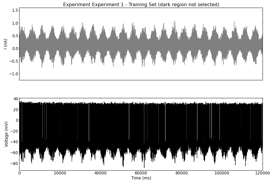
myExp.plotTrainingSet()
myExp.plotTestSet()
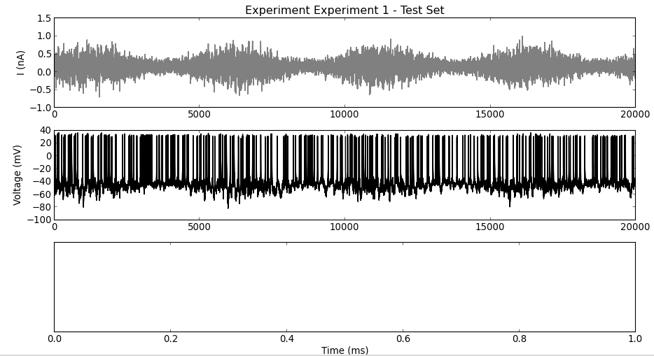
The responses to multiple frozen-noise injections are plotted on top of each others (middle). Since spikes have not yet been detected, the bottom panel is empty.